Spacecraft orbital tube monitoring

a_gior · April 5, 2024, 11:01am

Dear all,
I am currently trying to measure the effects of higher order perturbations and drag on the nominal trajectory of a satellite over 3 days. The method I am using is:

initialize the spacecraft state with its osculating keplerian orbit parameters
propagate the spacecraft state considering only gravitational perturbations up to a certain degree
propagate the spacecraft state with a different propagator, which considers higher order gravitational terms and drag
evaluate the position difference between the two satellites, centered in the LVLH frame of the nominal spacecraft.

In this way, I should be able to evaluate the relative position between the nominal trajectory and the perturbed one, and the choice of coordinates allows me to evaluate whether the real trajectory is within the boundaries of an orbital tube, centered in the nominal trajectory, with components on the across-track and radial direction.
The method I am using to compute at each time the LVLH frame of the nominal trajectory is taken from this thread.

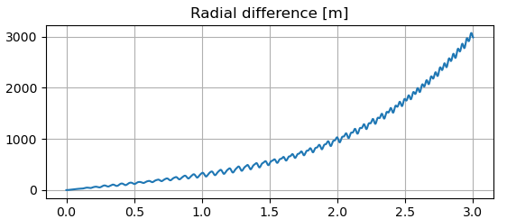
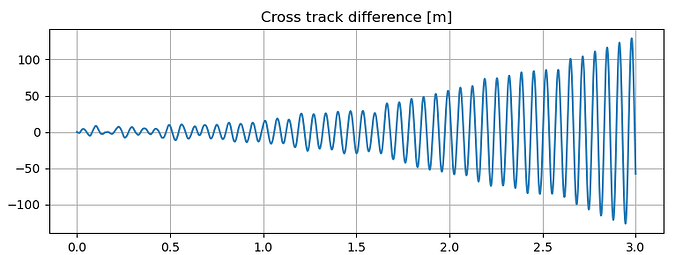
What I expect to see is a slight difference on the along-track direction, an oscillation for what regards the across-track direction and a constant increase for the radial direction, due to drag.

What I observe is that the component in the along-track direction rapidly diverges and reaches thousands of kilometers in a few days! The across-track component oscillates around 0 and the radial increases, which is something that I would expect instead (but I am not certain about the magnitude)

Here is the code that I am using, did I implement something wrongly?

year = 2026
month = 1
day = 1
hour = 6
minute = 0
seconds = 03.146
date_propagation = '2026-01-01T06:00:03.416'
utc = TimeScalesFactory.getUTC()                                                 
epochDate = AbsoluteDate(year, month, day, hour, minute, seconds, utc)           
epoch = Time(date_propagation)                                                     

duration = 3*24*60*60.                                                  # Propagation duration [s]


J2 = -Constants.EIGEN5C_EARTH_C20

h = 500e3  # Orbit altitude [m] 
R_e = Constants.WGS84_EARTH_EQUATORIAL_RADIUS 
a = Constants.WGS84_EARTH_EQUATORIAL_RADIUS + h  
e = 0.0  
mu_e = Constants.EIGEN5C_EARTH_MU
i = radians(60)       
omega = radians(90.0)                
raan = radians(0.0)           
true_anomaly = radians(0.0)     
inertialFrame = FramesFactory.getEME2000()

# Initial orbit definition
initialOrbit = KeplerianOrbit(a, e, i, omega, raan, true_anomaly,
                              PositionAngle.TRUE,
                              inertialFrame, epochDate, Constants.EIGEN5C_EARTH_MU)

period = initialOrbit.getKeplerianPeriod()
step_time = period/300                                                     # Propagation step-time [s]

satellite_mass = 70.                    # Spacecraft mass [kg]

# Numerical propagator definition - nominal
minStep = 0.001
maxStep = step_time
initStep = step_time
positionTolerance = 1E-2
propagationType = OrbitType.CARTESIAN
tolerances = NumericalPropagator.tolerances(positionTolerance, initialOrbit, propagationType)
integrator = DormandPrince853Integrator(minStep, maxStep, orekit.JArray('double').cast_(tolerances[0]), orekit.JArray('double').cast_(tolerances[1]))
integrator.setInitialStepSize((initStep))
numericalPropagator = NumericalPropagator(integrator)
numericalPropagator.setOrbitType(propagationType)
itrf    = FramesFactory.getITRF(IERSConventions.IERS_2010, True) # International Terrestrial Reference Frame, earth fixed
earth = OneAxisEllipsoid(Constants.WGS84_EARTH_EQUATORIAL_RADIUS,
                         Constants.WGS84_EARTH_FLATTENING,
                         itrf)
gravityProvider1 = GravityFieldFactory.getNormalizedProvider(20, 20)
numericalPropagator.addForceModel(HolmesFeatherstoneAttractionModel(earth.getBodyFrame(), gravityProvider1))
numericalPropagator.setInitialState(SpacecraftState(initialOrbit, satellite_mass))


# Numerical propagator definition - perturbed
tolerances2 = NumericalPropagator.tolerances(positionTolerance, initialOrbit, propagationType)
integrator2 = DormandPrince853Integrator(minStep, maxStep, orekit.JArray('double').cast_(tolerances2[0]), orekit.JArray('double').cast_(tolerances2[1]))
integrator2.setInitialStepSize((initStep))
numericalPropagator2 = NumericalPropagator(integrator2)
numericalPropagator2.setOrbitType(propagationType)
gravityProvider2 = GravityFieldFactory.getNormalizedProvider(60, 60)
numericalPropagator2.addForceModel(HolmesFeatherstoneAttractionModel(earth.getBodyFrame(), gravityProvider2))
numericalPropagator2.setInitialState(SpacecraftState(initialOrbit, satellite_mass))
crossSection_drag = float ( 2 ) # Cross section area used for drag
dragCoeff = 2.2 # Spacecraft drag coefficient

# Initialize drag perturbation
sun = CelestialBodyFactory.getSun()                                 # Create sun in simulation
strenghtLevel = MarshallSolarActivityFutureEstimation.StrengthLevel.STRONG
supportedNames = MarshallSolarActivityFutureEstimation.DEFAULT_SUPPORTED_NAMES
inputParameters_Drag = MarshallSolarActivityFutureEstimation(supportedNames, strenghtLevel)
atmosphere = NRLMSISE00(inputParameters_Drag, sun, earth)
spacecraftDrag = IsotropicDrag(crossSection_drag, dragCoeff)
drag = DragForce(atmosphere, spacecraftDrag)
numericalPropagator2.addForceModel(drag)

initialDate = epochDate
t = [initialDate.shiftedBy(float(dt)) for dt in np.arange(0, duration+step_time, step_time)]
spacecraft1 = [numericalPropagator.propagate(tt) for tt in t]  # Nominal
spacecraft2 = [numericalPropagator2.propagate(tt) for tt in t] # Perturbed

pv = [x.getPVCoordinates() for x in spacecraft1]
lvlh = [LofOffset(sc.getFrame(), LOFType.LVLH_CCSDS) for sc in spacecraft1]
converted_sc1 = [SpacecraftState(sc1.getOrbit(),  lvlh_list.getAttitude(sc1.getOrbit(), sc1.getDate(), sc1.getFrame())) for sc1, lvlh_list in zip(spacecraft1, lvlh)]

p1_along = [x.getPosition().getX() for x in pv]
p1_normal = [y.getPosition().getY() for y in pv]
p1_radial = [z.getPosition().getZ() for z in pv]

pv2 = [y.getPVCoordinates() for y in spacecraft2]

pv2t = [a.toTransform().transformPVCoordinates(y.getPVCoordinates(x.getFrame())) for a,y,x in zip(converted_sc1, spacecraft2, spacecraft1)]

pv2t_along = [x.getPosition().getX() for x in pv2t]
pv2t_normal = [y.getPosition().getY() for y in pv2t]
pv2t_radial = [z.getPosition().getZ() for z in pv2t]

plt.plot(np.arange(0, duration+step_time, step_time)/24/60/60, pv2t_along)
plt.title('Along track difference [m]')
plt.show()

plt.plot(np.arange(0, duration+step_time, step_time)/24/60/60, pv2t_normal)
plt.title('Cross track difference [m]')
plt.show()

plt.plot(np.arange(0, duration+step_time, step_time)/24/60/60, pv2t_radial)
plt.title('Radial difference [m]')
plt.show()

Another way I could perform my activity is to evaluate the variation in the keplerian parameters and derive the position difference from these, but I would like to maintain this approach, if possible.

luc · April 5, 2024, 11:34am

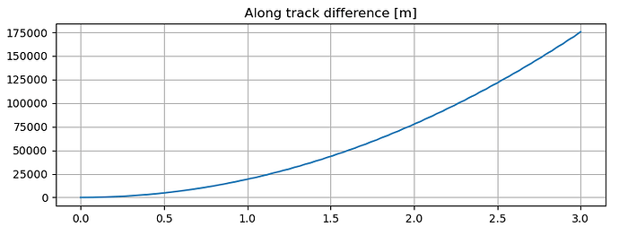
If you compare one orbit with drag and another without drag, it is expected that both the radial and along track differences diverge: drag does change the energy so semi major axis decreases and mean motion changes.

a_gior · April 5, 2024, 12:42pm

Dear @luc, thank you for you answer.
I agree with you that the decreasing semi-major axis changes the mean motion of the spacecraft, but is this meant to generate a difference of over 150km over three days on the along track direction?

I have a further question: would it then be possible to evaluate the difference between the two trajectories, evaluating at each time-step the intersection between the perturbed trajectory and the plane perpendicular to the nominal flight direction? In this way, I would be able to evaluate the deviation from the nominal trajectory without considering the along-track difference, but only accounting for the radial/across-track differences when the two trajectories are lying on the same plane.

If I compute the position difference as in the opening post, it seems that the perturbed satellite will move forward in the along-track direction with respect to the nominal one as the graph is showing: the position of the perturbed spacecraft CoM will be forward with respect to the nominal one, and the difference in position between the two is not computed “on the same plane” but at the same instant in time, for which the perturbed spacecraft finds itself forward with respect to the nominal one.

luc · April 5, 2024, 1:46pm

Just consider the Keplerian period of a satellite at 500km altitude and another one at 499km altitude. The first one is 5676.977s and the second one is 5675.738s, hence a difference 1.238 seconds. At an orbital velocity of 7613 m/s this means the two satellites are 9.4 km apart from each other after just one period. At slightly more that 15 orbits per day, you reach 150km pretty quickly. Drag at 500km altitude is important. I don’t know if it will drop the semi major axis one kilometer below on a few days, but you get the point.

It is possible to project trajectories to the perpendicular plane, but you will get nasty curvature effects. If you consider for example two satellites exactly at the same radius but one ahead of the other, then due to orbit curvature each one would appear to the other below its local horizon, hence they would have one negative Cartesian coordinate despite they are at the same altitude. Comparing orbits that are far from each other is not as straightforwar as it seems, everything is curved.

a_gior · April 5, 2024, 2:13pm

It is possible to project trajectories to the perpendicular plane, but you will get nasty curvature effects. If you consider for example two satellites exactly at the same radius but one ahead of the other, then due to orbit curvature each one would appear to the other below its local horizon, hence they would have one negative Cartesian coordinate despite they are at the same altitude. Comparing orbits that are far from each other is not as straightforwar as it seems, everything is curved.

I agree that this would happen if one projects the trajectory of one satellite onto the perpendicular plane of the other, but I guess this should not happen if I consider the intersection between the perturbed trajectory and the plane, not its projection.

Is there an easy way to perform this task? I am thinking about generating such plane using the position/velocity of the nominal spacecraft, and then interpolate between each position vector of the perturbed one until an intersection is found… but maybe there is an easier way already implemented.

EDIT: I am trying the above and with the help of hipparchus I am able to define the plane perpendicular to the flight direction and to define a straight line between each position of the perturbated spacecraft, and to find the intersection between the two. Using also the above definition of “converted_sc1”, how can I express this intersection point (Vector3D) in the local reference frame of the nominal spacecraft?

a_gior · April 8, 2024, 1:54pm

Dear @luc , sorry to bother you again.
I have managed to use hipparchus “Point”,“Line” and “Plane” in order to obtain the objects I need to generate the plane perpendicular to the nominal spacecraft at a given propagation index, and then interpolate between the propagated positions of the perturbed one in order to find the intersection with the given plane. Such intersection point is obtained as Vector3D.

What I am missing now is to express the position of this intersection with respect to the local LVLH of the nominal spacecraft: I have access to “converted_sc1” as mentioned in the opening post, which should contain the information relative to the LVLH frame at each timestep and I can extrapolate the one I need given the time-step at which I am generating the plane.

I am missing how to express the transformation from ECI to LVLH, since if I use:

lvlh_point = converted_sc1[index_plane].toTransform().transformPVCoordinates(p_intersection)

it fails since transformPVCoordinates needs PVCoordinates, and p_intersection, coming from Intersection in hipparchus, is a Vector3D (which should be in ECI, since everything is performed from vectors taken from PVCoordinates.getPosition()).
How can I obtain this position in LVLH?

EDIT: I have managed to obtain what I want, but strangely the intersection point that I find does have a small component on the along-track, when I translate the intersection to the LVLH of the nominal satellite… ideally it should be 0.
I have implemented the procedure in the following way, with index_plane as the index of the nominal satellite and sat2_index as the indexes of the perturbed satellite:

plane_1 = Plane(pv[index_plane].getPosition(), pv[index_plane].getVelocity(), 0.001)  # define current nominal satellite plane. Plane defined with point of sat1 position and normal to its velocity
line_int = Line(pv2[sat2_index].getPosition(), pv2[sat2_index-1].getPosition(), 0.001) # Try to find intersection between perturbed satellite and nominal plane, define line between propagated points
p_int = plane_1.intersection(line_int) # Find intersection
point_nom = pv[index_plane].getPosition() # Position of nominal satellite
dist = Vector3D.distance(p_int,point_nom) # Find distance between intersection and nominal satellite
lvlh_point_int = StaticTransform.cast_(converted_sc1[index_plane].toTransform()) # Use converted_sc1 to define transform at given timestep to LVLH 
lvlh_point = lvlh_point_int.transformPosition(p_int) # Transform intersection to nominal spacecraft LVLH
along_int = lvlh_point.getX() # Along track component
across_int = lvlh_point.getY() # Across track component
radial_int = lvlh_point.getZ() # Radial component

The way I define the plane at line 1 should be the same as the plane definition in LVLH_CCSDS… or am I missing something?

luc · April 11, 2024, 7:33am

I don’t really get why you use plane and line. Wouldn’t you get the same across_int and radial_int coordinates by just looking at the Y and Z components of lvlh_point_int.transformPosition(pv2[sat2_index].getPosition())?

When you say you have a small component along track, what is the value of small? Is it some numerical noise at micrometer level or is it larger?

a_gior · April 11, 2024, 9:55am

Dear @luc , the reason why I am currently using plane and line is because of the effect you have mentioned in your first reply: since I need to evaluate the radial/across-track error between the two spacecraft on a plane perpendicular to the flight velocity of the nominal satellite, I can’t just perform the difference between the two positions at the same instant of time. As you have mentioned, one spacecraft will be in front of the other, and this would cause a difference in the radial component and, as the propagation goes on, I would be comparing two spacecraft that will be far away from each other while I need to monitor their trajectory relative to the nominal one, orthogonally with respect to the velocity of the nominal spacecraft.

I have managed to solve my issue on the component along track, and it seems it was caused by the definition of the plane. I was generating the plane using the position vector of the nominal spacecraft and its velocity as the normal of the plane: with this definition, I obtained along-track components in the range of tens of centimeters. I have checked the definition of LVLH_CCSDS and I have found that it is defined with the position and the orbital momentum of the spacecraft, so I changed the definition of my plane to:

v_lvlh = Vector3D.crossProduct(pv[index_plane].getPosition(),pv[index_plane].getMomentum().negate())
plane_1 = Plane(pv[index_plane].getPosition(), v_lvlh, 0.001)

and now I am finding along-track values in the range of 1E-10 meters.

Everything seems to work fine like this, but references suggest that I should be getting a parabolic across-track component error which should be continuously increasing with time, while mine seems to be bounded and I can not find the reason why… since the radial component seems to be correct

a_gior · April 12, 2024, 4:11pm

Hello @luc , sorry to bother you again.

I am still struggling with this issue: as I have told you, I have managed to generate planes (perpendicular to the flight direction) for every timestep of my nominal satellite and I have found the intersection between each plane and the trajectory of the perturbed satellite, which has been propagated with much smaller time-step.

The end result is:

a null component in along-track, which is expected since each intersection lies on the plane by definition
an increasing radial component, which values are representative of what equations from theory provide
an oscillating but bounded across-track component, which should be oscillating but increasing in altitude with the shape of a parabola.

From theory, the across-track component at ascending node is dependent on semi-major axis, inclination and shift in ascending node longitude. I have computed the ascending node longitude for both satellite at each respective equator crossing, finding a parabolic behavior which in result gives me a parabolic (theorical) shape for the ascending node across-track error. So I really can not understand why using positions instead of the ground track I am not seeing the same effect on the across-track, while theorically (using the propagated delta-lambda) I am seeing it.

I really can’t seem to find what I could be implementing wrongly. This is what I am currently using as code, in which “index_plane” stands for the propagation index of the nominal spacecraft, while index2 is the index of propagation of the perturbed one.
As mentioned earlier, I have defined such plane using the velocity not directly obtained from propagation, but calculated through the angular momentum since I was obtaining some components in the along-track while converting the intersection of the plane to LVLH_CCSDS (which is defined based on position and angular momentum).

for index_plane in indexes_plane:
    print('new plane')
    v_lvlh = Vector3D.crossProduct(pv[index_plane].getPosition(),pv[index_plane].getMomentum().negate()) # velocity for plane generation
    plane_1 = Plane(pv[index_plane].getPosition(), v_lvlh, 0.001) #current plane
    pnew = pv2[index_good].getPosition() # position of spacecraft2
    off_new = plane_1.getOffset(pnew) #offset of position of spacecraft2 wrt plane
    for indexes2 in np.arange(index2_new+1, index2_new+10000, 1): # start from next position
        off_old = off_new
        pnew = pv2[indexes2].getPosition() # new position of spacecraft 2
        off_new = plane_1.getOffset(pnew) #offset of position of spacecraft2 wrt plane
        if off_old*off_new < 0: #if points lie on different side of plane
            line_int = Line(pv2[indexes2].getPosition(), pv2[indexes2-1].getPosition(), 0.001) #generate line
            p_int = plane_1.intersection(line_int) # find intersection
            off_int = plane_1.getOffset(p_int) #check offset of intersection (shall be 0)
            point_nom = pv[index_plane].getPosition() # position of nominal spacecraft
            dist = Vector3D.distance(p_int,point_nom) #distance between nominal spacecraft and intersection of spacecraft2 trajectory
            lvlh_point_int = StaticTransform.cast_(converted_sc1[index_plane].toTransform()) #transformation intermediate step
            lvlh_point = lvlh_point_int.transformPosition(p_int) #transform intersection to LVLH of spacecraft1
            along_int = lvlh_point.getX()
            across_int = lvlh_point.getY()
            radial_int = lvlh_point.getZ() 
            index2_new = indexes2
            dist_vec.append(dist)
            along_vec.append(along_int)
            across_vec.append(across_int)
            radial_vec.append(radial_int)
            break

I have also implemented the solution of checking the perturbed satellite position with respect to the LVLH at the same steps, but as a result I got, as expected, a component in the along track and a much higher component in radial (due to the fact that the perturbed spacecraft is in front of the other). The across-track component still remained oscillatory and bounded with the same values I got with the plane method.

luc · April 12, 2024, 9:34pm

I wonder if you are not stuck with the difference between osculating and mean parameters.
Theories often rely on very simplified equations and are expressed in some kind of mean parameters (which depend on the theory) that remove all short period terms. When dealing with classical propagation, like numerical propagation for example, you get all these harmonics back.
In some cases, harmonics are really huge, see for example this thread and the eccentricity plot, in this case the short period terms are larger than the mean elements. Perhaps as you pick several points around the orbit you see short periods?

a_gior · April 15, 2024, 10:40am

Dear @luc, thank you for your suggestion and the interesting read on your thread.

The cross-track error equation I have found at ascending node is [S. D’Amico, M. Kirschner, and C. Arbinger. Precise orbit control of leo repeat observation satellites with ground-in-the-loop. case of study: Terrasar-x. German Space Operations Center (GSOC) TN 04-05, 02 2004.]:

in which:

r represents the semi-major axis of the nominal spacecraft trajectory
dLambda is the difference in longitude at ascending nodes between the two satelites
i represents the orbit inclination of the nominal satellite
alpha_0 is the angle between the flight velocity of the nominal satellite expressed in ECEF and ECI (this is approximated with 3.7° for LEO)

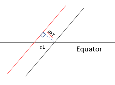
This equation is coherent with this image, in which I have represented the across-track distance as dXT, which can be obtained as shown earlier using dL (longitude difference at the ascending node), the sine of the inclination and then by multiplying by the semi-major axis:

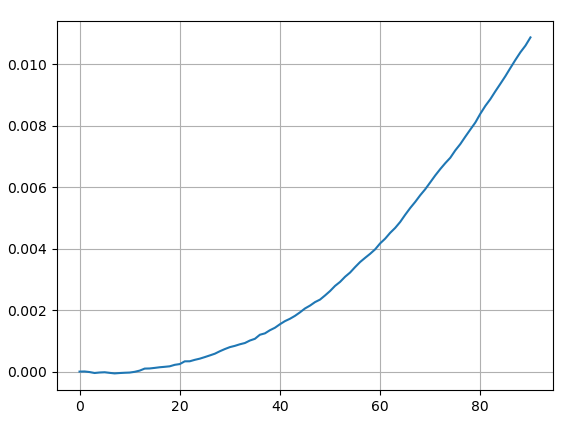
When I try to plot the delta-longitude evolution of the ascending nodes I do indeed obtain a parabolic behaviour (x- axis: #orbit, y-axis delta-longitude in degrees)

The evolution of delta-longitude of ascending nodes, obtained by propagating both satellites with osculating elements, is representative of the parabolic behaviour expected with time which is mentioned in several references.
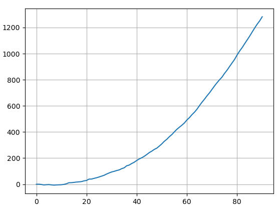
I can then by using the equationto evaluate the expected across-track error at each ascending node (x-axis: #orbit, y-axis: across-track error in meters)

Simple geometry is suggesting me that I should be seeing a parabolic behaviour (at least at ascending node), but the method I am using with the planes and the translation to LVLH is failing… and this happens only on the across-track component, because the radial component follows the behavior I expect to see. I am sampling each orbit with over 500 planes so even though at each orbit the plane is not exactly at the ascending node, I am really close to it within +/-1° of true anomaly.

I understand that the variations in the osculating elements may cause some differences, but such differences are small when compared to the results I should see (parabolic behavior vs bounded one), at least for a few days of propagation. Furthermore, since the delta-longitude I obtain with the propagation of osculating elements is what I expect, I believe the error is probably lying in the plane/LVLH definition, but from the code I posted above I can not see where the error could be.

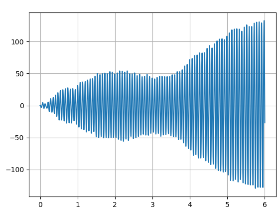
The error I obtain on the cross-track by using the plane method is the following (x-axis: #days of propagation, y-axis: cross-track error in meters): one day should reflect around 15 orbits, to compare with the previous graph

luc · April 15, 2024, 12:07pm

Is your eccentricity properly frozen?
Look at equation 3.18 in paper Very Low Thrust Station Keeping for Low Earth Orbiting Satellites, it shows that longitude offsets are affected by many parameters (in fact all orbital parameters). I wonder if you are not seing the pulsating effet due to eccentricity. If eccentricity is slightly different from the frozen one, the perigee will slightly wander with respect to the expected nominal one. This implies at some points your satellite is ahead of its nominal position and at some points it will be behing its nominal position. Hence it will be either early or late with respect to Earth rotation, and this results in an oscillating East-West discrepancy, even if semi-major axis is good (i.e. if mean motion is correct).

a_gior · April 17, 2024, 8:25am

I have managed to find the solution: the LVLH frame is not perfectly aligned with velocity (being constructed based on position and angular momentum). If I define manually a frame that is aligned with position and velocity, I see the effect that I was looking for.