It is used, but not as a tube. What is used is delta-longitude on a grid.
If you have for example a drift in semi-major axis due to atmospheric drag, the orbit period will decrease and the track will globally shift eastwards, hence looking at the shift is used to maintain semi-major axis.
If you have a change in inclination, the track will skew, with the northern part going eastwards and the southern part going westwards, or the opposite depending on sign of inclination change.
If you have a change in eccentricity, the track will also skew as part of the orbits will be traveled faster (hence eastwards shift with respect to Earth rotation) and other parts will be traveled slower.
In theory, you could use the grid track to control all parameters, but often the inclination part is controlled using local solar time for Sun Synchronous Orbits, and the track in ECEF is used for maintaining semi-major axis, but I have not seen using a tube.
Dear @luc,
thank you for the insight! I guessed that typically an orbital tube is not used, but I need to do it since my application is similar to the one reported here.
I still have a final question though: is it possible to control at the same time the ground-track drift and the along-track shift? Ideally, both show a parabolic behaviour due to drag: the ground-track is as you explained, while the along-track position shifts forward if the semi-major axis is lower and backwards if it is higher after a manoeuvre.
When correcting the semi-major axis both are affected, but at the current state I am able to control only one at a time, with the other component showing the expected evolution until some divergence arises due to accumulated error. Is there a strategy typically used to ensure that not only the longitude drift is maintained, but also the along-track position, which affects the timing of the trajectory?
Both along track and longitude are linked together. If you get the longitude OK, the timing will be OK, but this requires the ground track to be really accurately defined. In the paper I mentioned earlier in the thread, there is a method proposed to set up this grid. It mainly consists in first have a rough grid, computed with simple means (like the Phasing tutorial) and no drag, and then to iterate with a station-keeping simulation software and taking into account both drag and the maneuvers that compensate it. Then, computing the median of the station-kept track, you finally end up with something that is both stable and representative of everything that really happens to the spacecraft.
This final track will be synchronized both in longitude and along track.
Dear @luc, many thanks for the insightful details on the topic. I agree that for real-world station-keeping it is important to define the grid in a way that is representative of reality also taking into account manoeuvres and generating the grid as a median of all passes. In my case, this would translate to a list of ECEF-defined SpacecraftStates.
I was wondering though, if it is possible to still obtain a reasonable estimation of station-keeping manoeuvres frequency and budget (in-plane and out-of-plane) even by just using as “reference orbit” what is obtained through orekit when using a NumericalPropagator with only Earth’s gravitational harmonics.
With your suggestions, I have implemented the evaluation of the relative position between the reference trajectory and a perturbed spacecraft and when (only one of) along-track or across-track boundaries is exceeded, a manoeuvre is triggered (references suggest minimization of eccentricity vector difference for the manoeuvre location). I have implemented it in this way since I thought that given that both show a parabolic behaviour over time, whenever I correct the most stringent objective (in my case, along-track), the across-track distance is maintained too within its boundaries and should show a parabolic behaviour within a smaller control band. What is happening instead is that some offset builds up in the non-controlled direction, while the other remains within its boundaries, and therefore the across-track (or ground-track) is not maintained if I focus only on the along-track timing.
Is there actually no other option other than performing the procedure you mentioned, applying the median on the trajectory for several (controlled) repeat cycles? While I agree that it might be necessary for a very good estimation of real-life operations, I was wondering if it was possible to still show obtain a reasonable delta-v budget for station-keeping with a simpler reference trajectory. Maybe I am missing something in my control concept, is there a tutorial for ground-track maintenance within Orekit, that also takes into account along-track shift (timing)?
Dear @luc ,
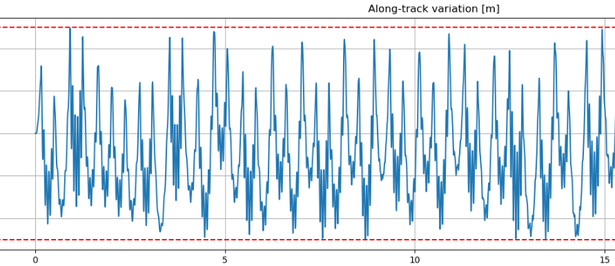
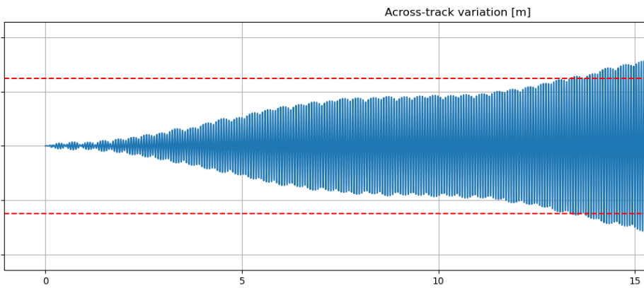
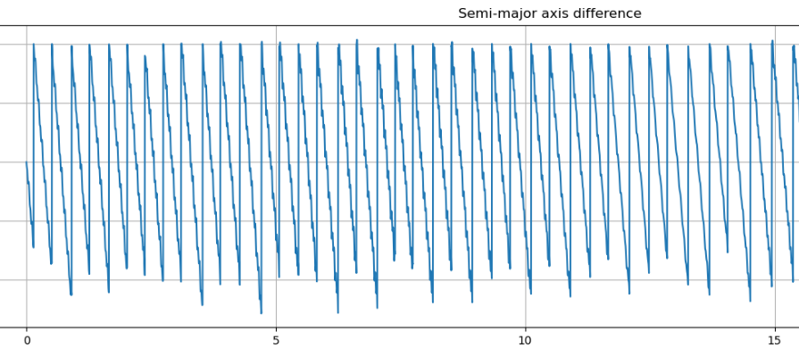
I think I might have found something to help me. I reported below the evaluation in ECEF (performed with your method) of the along-track and across-track distances. As it can be seen, the along-track diverges much faster and that is the reason why I am controlling it. I was expecting to be able to also control at the same time the ECEF across-track difference, which shows the parabolic behaviour I expect but with an increasing offset over time, with on top the parabolic behaviour. I have also reported the semi-major axis variation.
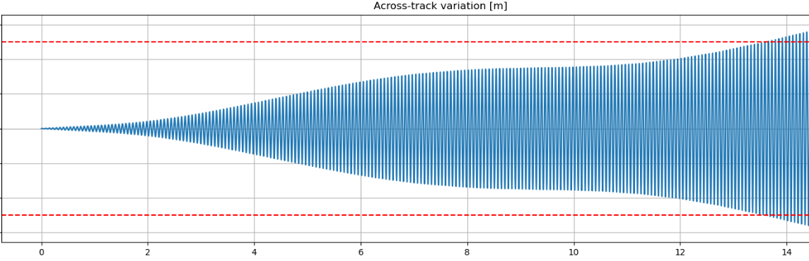
But I have just noticed one thing: if I try to plot the ECI across-track difference between the two spacecrafts, I obtain this behaviour which actually looks like the offset between what I expect to obtain in ECEF.
    lvlh = [LofOffset(sc.getFrame(), LOFType.LVLH_CCSDS) for sc in spacecraft1]
    converted_sc1 = [SpacecraftState(sc1.getOrbit(),
                                     lvlh_list.getAttitude(sc1.getOrbit(), sc1.getDate(), sc1.getFrame())) for sc1, lvlh_list in zip(spacecraft1, lvlh)]

    pv3t = [a.toTransform().transformPVCoordinates(y.getPVCoordinates(x.getFrame())) for a,y,x in zip(converted_sc1, spacecraft3, spacecraft1)]
    pv3t_across_ECI = [x.getPosition().getY() for x in pv3t]
I am just adding SRP and luni-solar attraction as perturbing forces other than drag, but should I see such big variation in a short amount of days in ECI? The ECEF difference looks like the parabolic behaviour I expect, summed with the ECI one… so does this mean that this could come from a very big rate change in inclination, that I shall correct sooner? Even though the shape of the inclination change does not exactly follow the across-track variation (and I believe the latter should look like a*delta_i)
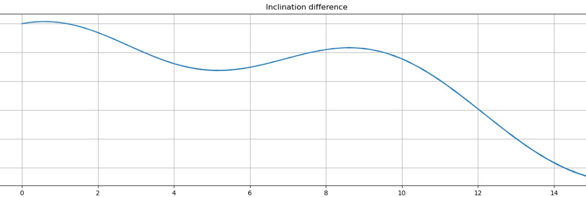
EDIT: it seems that keeping only drag and SRP gives back a linear trend of inclination difference, and the evaluation of a*di matches the ECI across-track difference… probably the luni-solar attraction has relevant effects on the other parameters too?
I am not sure I understand all the side effects of working in ECEF.
Concerning luni-solar effects, yes they have an influence on orbital plane (they change inclination), hence the points in ECEF on North hemisphere drift in one direction and the points on South hemisphere drift in the other direction.
Dear @luc , I think I have found the culprit.
Yes I agree that the ECEF reference can be misleading, in fact now I’m trying to work in ECI only to understand changes in the inertial frame.
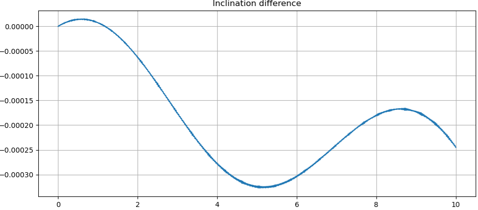
When only implementing drag and SRP, the inclination decreases linearly over time generating an across-track difference at maximum latitudes. If I correct that inclination difference, the relative across-track distance goes to 0 as expected.
If I implement also luni-solar attraction, the inclination difference shows an higher magnitude difference: furthermore, if i try to correct it, only a small change with respect to the overall across-track distance is seen, leaving still a big error behind.
If I also look at the raan difference, I see this behaviour that is exactly following the shape found in the across-track axis (both ECI and ECEF). Values are in degrees.
raan1 =np.array ([np.degrees( np.arcsin(x.getHy()/np.tan(x.getI()/2)) ) for x in spacecraft1])
raan2 =np.array ([np.degrees( np.arcsin(x.getHy()/np.tan(x.getI()/2)) ) for x in spacecraft2])
draan = raan2-raan1

If I try to manually evaluate the across-track error at nodes (ECI) due to raan difference using a* draan*sin(i) I obtain the exact value of across-track error that I see in ECI too, for a generic altitude of 500km and mid-inclination of 45°.
If I also try to manually evaluate the delta nodal precession between the two, using the delta-inclination found, the RAAN variation seems very high to be caused by nodal precession only.
Does this mean that the luni-solar third-body attractions are directly highly modifying the RAAN, and therefore I should consider RAAN correcting manoeuvres too? I was not expecting this big effect of luni-solar attraction in LEO.
To be honest, I don’t know.
Dear @luc,
in the end I managed to also implement RAAN correction manoeuvres that do indeed manage to correct the across-track difference that I was noticing when implementing luni-solar third body attraction.
I have one question regarding the set-up procedure I am implementing in the propagators: up to now, to measure the differences due to drag/SRP/luni-solar third body attraction I was using the same order/degree for the gravity field provider (12x12) in the following way:
- initialize mean keplerian parameters
- create DSST propagator with 12x12 gravity field as only active force
- generate osculating state from mean DSST propagator state and 12x12 gravity field
- create “nominal” numerical propagator (without drag/SRP/luni-solar) and with 12x12 gravity field and initialize the initial state using the osculating state
- create “perturbed” numerical propagator with drag/SRP/luni-solar and 12x12 gravity field, initialized with the same osculating state
In this way, the harmonics used are the same and I am able to see the differences due to other perturbations.
If I now modify the degree/order of the field of the “perturbed” propagator, but maintaining the same initial osculating state from the previous steps (12x12 nominal field), I start noticing very big differences in the osculating differences of the keplerian parameters, and not small oscillations around the values I was obtaining before. This happens already if I use a 13x13 gravity field for the “perturbed” propagator, while the other stays at 12.
The only way I am able to reproduce the values I was obtaining with equal gravitational fields is if I adopt something like a 60x60 field for the “nominal” propagator and 120x120 for the “perturbed” one, but this of course heavily increases the computational time. If I try to decrease the nominal back to 12x12, using 120x120 for the perturbed the differences are too high.
So my questions are:
- first of all, is my method of initializing the two propagators correct, using the same initial osculating state computed through the “nominal” propagator?
- if in the end I am obtaining very similar values between 12x12/12x12 and 60x60/120x120 combinations of nominal/perturbed, wouldn’t it be beneficial to maintain the first case? I guess that I will lose information on the effect of higher order harmonics in this way. In the second case, I am using two trajectories that require much more time to compute.
I understand that, as you mentioned earlier, the “nominal” trajectory is obtained after optimization of several repeat cycles. Nevertheless, I wanted to still be able to have a measure of delta-v/frequency of station-keeping manoeuvres even with a simple propagated nominal orbit.
Regards.