Hi @bdruby, welcome onboard
Your observation is correct, and it is a normal behaviour.
Many angles in space flight dynamics can evolve over time without limitation. True/Mean/Eccentric anomaly is the best example. When computing Keplerian elements from Cartesian elements, the algorithm used in Orekit is to compute the orbital plane (which is orthogonal to to orbital momentum given by the cross product of position and velocity), then to compute the semi major axis using equation of energy which depends on position and velocity modules only, then to compute both the relative position of satellite with respect to apogee/perigee and the eccentricity using basically the angle between position and velocity, thus getting the true anomaly, and finally to deduce argument of perigee by getting the angle between the current position and the node that was computed when orbital plane was computed at the beginning, and subtracting the true anomaly obtained before.
So as a summary, as you said when computing Keplerian elements from Cartesian elements, argument of perigee is obtained from a subtraction between two angles that are themselves computed using atan2, hence both lie in the [-π ; +π] interval. The result of the subtraction can therefore reach any value in the [-2π ; +2π] interval.
Once an orbital state has been converted from Cartesian elements to Keplerian elements, the values of these elements will evolve as soon as you take into account any perturbations, so the angles obtained before are only initial values. Many of the angles may drift indefinitely and make several turns. Of course, the faster angle is anomaly which makes one turn every orbit (but wait for the fun fact below). In order to avoid numerical problems and simplify computations like smoothing using running averages or computing rates using finite difference, Orekit does not normalize this angle back into some canonical interval, neither [0; 2π] nor [-π ; +π]. So even if you start with a small angle, after several orbits you may well have a true anomaly of several thousands radians. This is normal and the equations behave properly with large angles (as a side note, in numerical analysis one should never normalize an angle back to small values before computing its sine, cosine or tangent, one should call the mathematical function using the big angle as the argument reduction done internally is much more accurate that what you would do by yourself, so keeping the big angles also improves accuracy).
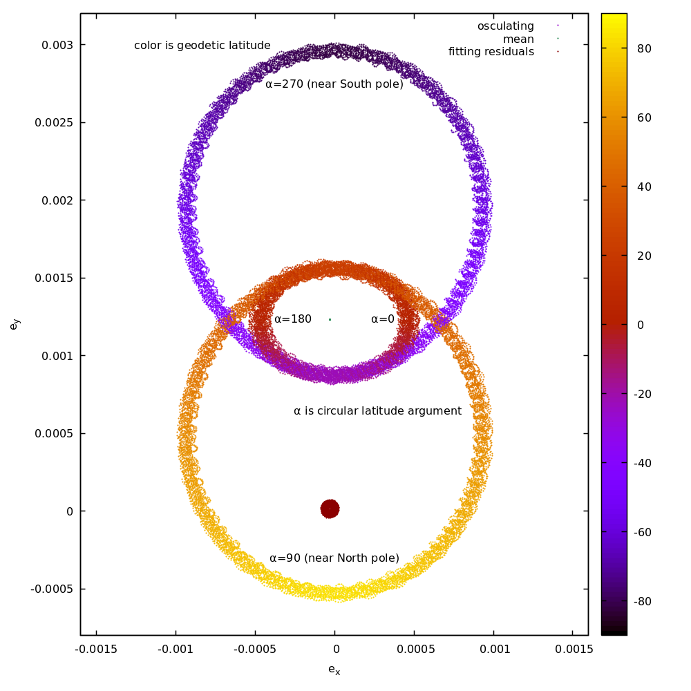
If you consider for example an observation satellite, the operational orbit is often selected in such a way the right ascension of the ascending node Ω will also drift indefinitely, at a smaller rate than anomaly, but after one year it will have made one full turn, so this angle too may end up with values outside of canonical intervals. Inclination will never do full turn (well theoretically it could using maneuvers, but I have never seen any operational mission needing such weird and costly behaviour), and as by convention it is always computed using the ascending node as a reference, it remains in fact constrained in the [0; π] interval. Argument of perigee ω is not constrained, and just as Ω it may drift. A fun fact is that if you look at osculating parameters for an orbit with frozen mean perigee, then the osculating perigee moves around the orbit following (in circular parameters) an elegant figure-8 shape that could contain the (0, 0) origin:
This plots shows the eccentricity vector (e cos(ω), e sin(ω)) evolving over time for such an orbit, in
osculating elements. This is a single curve, the color code represents the geodetic latitude. The eccentricity vector follows the full curve each orbit, so you see that if you start the orbit at latitude argument α = 0 (i.e. crossing equator from South to North), eccentricity is as the right hand side of the small oval, which is in the red part because latitude is 0. Then satellite goes North up to its maximum latitude at α=90° and follows the lower part of the curve counterclockwise, so esin(ω) get its minimum value (about -0.0005 in this plot), in the yellow part because latitude is positive, this takes one fourth of the period. Then the satellites goes South again to reach the descending node at α=180°, finishing the lower part of the plot and back in the red region as it again approaches equator. Then it performs the part of its orbit in South hemisphere, traveling in the upper purple region (because latitude becomes negative), with α going to 270° near South pole and back to 360° when finishing the orbit. As you see, during this orbit the osculating eccentricity vector (e cos(ω), e sin(ω)) has made one full turn around the origin (0,0), which means ω has made one full turn in the [0 ; 2π] interval. In this example, the argument of perigee (osculating!) moves around the orbit. As a side effect, the latitude argument does
not drifts indefinitely anymore! It just oscillates. So in this case it is not the satellite that crosses its perigee once per orbit, it is the perigee that crosses the satellite once per orbit and ω can reach values far outside of the [0; 2π] interval, it could reach thousands of radians too.
I agree, this is an extreme case, but it is a real one and used in many operational satellites. It also mainly shows that Keplerian elements are not the good choice for such orbits, circular elements (i.e. eccentricity vector and latitude argument) are better suited here than argument of perigee and anomaly.
So as a summary, you are right, argument of perigee can be outside of the [0 ; 2π] interval, but it is normal. There are no reasons why it should be bound to this interval. There are on the other hand numerical reasons for not normalizing it back during computation (but it is OK to normalize when writing down to files for example) and there are also physical reasons why the angle once computed may drift indefinitely.
 That is a great plot. Did you just make it?