SOCIS 2019: Orbit Determination with SatNOGS

Hi all,

I am working on the SOCIS 2019 project with the aim of determining the feasibility of using the Doppler shift of a satellite transmission to determine its orbit.

The idea is that the resulting system should be able to use Orekit and a satellite’s TLE to produce an initial estimate of the orbit of the satellite (this is already possible) along with the theoretical Doppler shift that would be observed at a given ground station.
The Doppler shift that is measured by the SatNOGS receiver could then be used to refine the estimated orbit by minimising the residuals between the estimated and measured doppler shifts for that ground station.

I received some data for the Max Valier satellite from the SatNOGS team and have written a script to convert the frequency measurements and corresponding MJD data to a format that can be utilised by the Orekit determination program. The current most up to date version of this converter is on the forge.
As of today the sign convention on the range-rate conversions have been changed to follow those used by Orekit (negative when the satellite is approaching and positive when moving away.)

I have also carried out a first series of orbit determinations using the Doppler curves provided by SatNOGS. This estimation run yielded large RMS error values, but this could arise from errors in setting the standard deviation in the configuration file (with the Standard deviation being set far too small when compared to the residuals, thereby causing the programme to reject all measurements as outliers.)

Regards,
Noël Janes

Hi @noeljanes,

In order to avoid the Orbit Determination to reject all measurements even if standard deviation setting is wrong, you may attempt to postpone outliers rejection until several iterations. Look at the range.rate.outlier.rejection.starting.iteration, which is currently set to 2. Set it to 10 for example so you get a chance to perform 10 iterations before rejecting measurements. Perhaps at this time the RMS would have had a chance to become more realistic.

Another point: you should remove the various polynomial.acceleration parameters in this case. They are suited for very special cases or very accurate (centimeter level) orbit determination.

Hi Luc,

I initially set the range.rate.outlier.rejection.starting.iteration to be 10, but unfortunately this didn’t reduce the size of the RMS values, but I did observe smaller ΔP and ΔV values suggesting that the program was converging on a fit, so I set it to 15 and got the following result:

The ground.station.range.rate.sigma is currently set to 0.001, while the ground.station.range.rate.bias is set to 0.

Thanks for the advice, I have removed the polynomial.acceleration parameters.

EDIT: Would it be possible to bring in the estimated values generated by the script you sent me to use them as the initial orbit guess?

Things are improving but we the measurements are still very far from what we expect and once the outliers rejection is triggered, it rejects everything.
Before rejecting, the batch least squares tries to estimate something. It moves the orbit, but not a lot. Looking farther in the output, it seems to select to change the drag coefficient and ends up at almost 61000 which is not realistic (except if the satellite deploys some parachute :wink: A classical value should be around 2.0. Note that drag uses drag.area, which is set to 0.25m² and seems realistic for this satellite, and it also uses mass which is commented out so the realistic value of 16 kg is not used and is replaced by the default 1000kg mass. Removing the hash character to uncomment mass will improve things, but not enough.

Could you try also increasing ground.station.range.rate.sigma a lot (say up to 1000.0) to see what happens? I have unfortunately no idea of the expected sigma for these antennas, it will mostly be an output of this study.

What do you mean by bringing in the estimated values as an initial guess? The script just generate simulated measurements, that you could try to use as measurements files (except you should remove the mjddate that is not used in the OD program). The initial guess is just the same as you use: a TLE in this case.

I hadn’t noticed that change in the drag coefficient :sweat_smile:

I initially ran the program again after just having uncommented the satellite mass and got the following results:

This gives a slightly less absurd change in the drag coefficient (although still orders of magnitude greater than expected as you said.)

Could you try also increasing ground.station.range.rate.sigma a lot (say up to 1000.0) to see what happens?

I tried this (I did have to raise the estimator.max. coefficients to 50 to get more than just an error message out of it.) The results are below:

Interestingly it doesn’t seem to make that much of a difference if the ground.station.range.rate.sigma is set to 100 or 1000, with the drag coefficient at sigma=100 being +5513.408923461590
(compared to drag coefficient=+5513.408922471820 at sigma=1000)

The last run is interesting, it does converge while keeping all the measurements. It also gives an interesting output value: the standard deviation on range-rate measurements is about 150m/s. This is a value we could now use the configuration sigma in the maxvalier.in file: we got our first result!

This value is very high for Orbit Determination needs and could explain why parameters estimation is weird, including drag coefficient. From a technical point of view, this is not surprising, though: the signal acquisition process for SatNOGS was not designed to perform Doppler measurements, its accuracy is sufficient for locking the signal so there was no reason for the designers to improve this. Our use as an orbit determination measurement is a trick to exploit a by-product of signal acquisition.

There are two things I would suggest to do now.

The first suggestion would be to try to retrieve and plot all the residuals, to see if we get something that look like a random noise around the zero line (which would be good and mean we did converge to something sensible) or if we see some regular pattern which would mean that we missed something and did not extract all possible information from these measurements.

If we see random noise in the middle and high noise or patterns near station acquisition of signal and loss of signal, this would still be normal. It seems the pass started almost at horizon and ended almost at horizon, so the first and last measurements have bee performed on very low elevation and are much more affected by atmosphere than measurements in the middle of the pass when the satellite is high. During operational orbit determination, measurements below about 5° elevation are generally dropped in a pre-processing phase.

As you maxvalier.in file has an entry output.base.name = orbit-determination, the orbit determination process should create in your home directory some output files, and in particular orbit-determination-range-rate-residuals.out (files for all measurements types are created during the run, and the ones that are still empty at the end because there are no measurements of this type will be automatically deleted, but the file for range-rate should remain). Could you plot the residuals (or upload the file if you don’t have a mean to plot it due to the format of the time field)? The file only contain the results after convergence, but if needed we could modify the code so we create one such file at each iteration, it is not difficult.

The second suggestion would be to modify the measurement generation program I sent to you, replacing:

            final RangeRateBuilder     builder      = new RangeRateBuilder(null, station, false, 0.0, 1.0, os);

by

  final double               sigma        = 150.0; // the value we will tune
  final RealMatrix           covariance   = MatrixUtils.createRealDiagonalMatrix(new double[] { sigma * sigma });
  final CorrelatedRandomVectorGenerator crvg =
    new CorrelatedRandomVectorGenerator(covariance,
                                        1.0e-10,
                                        new GaussianRandomGenerator(random));
  final RangeRateBuilder     builder      = new RangeRateBuilder(crvg, station, false, sigma, 1.0, os);

Then, running the measurements generation program, we will get simulated measurements that we could use to performed an orbit determination based on these measurements and see how it works. We would iterate on this, regenerating measurements and performing orbit determination using different values for the range-rate sigma. This would help us determine what value for sigma we need if we want to be able to do a reasonable orbit determination on a given number of passes. Beware that the measurement generation is performed on one station over one day. If we want to do a reasonable study, we should run it on several stations to have a more realistic configuration, and play on the number of passes we use.

There is however one problem with this suggestion: the orbital models in the orbit generation and in the orbit determination are not the same, but the initial point is the same. In a real operational case, it would be the opposite: we would have our orbit determination model as close as possible to reality but we would not know the exact initial orbit. We could address this by changing further the measurements generation program, but we can do a first try as is and see what we get. It would be interesting to look at results with a signma set to 150m/s, then 10 m/s, then 1 m/s, then 0.1 m/s. As the orbit models are different, we will not end up with a perfect orbit determination even with perfect measurements, but we will see what happens.

Perhaps you could also point the SatNOGS team to this thread and your current results and ask them right now if they think it would be possible to improve the accuracy of the Doppler measurement.

I have plotted the residuals for a sigma of 150 as you requested and have attached it below. It shows two peaks due to the two passes over the stations (the first at roughly 20:00 and the second at 21:30,) but neither appears to be random in the middle of the data. Could this be that I have plotted it incorrectly or is this something we’ve missed previously?

I have attached the residuals file as well for reference:
orbit-determination-range-rate-residuals-Sigma150.out (93.1 KB)

Edit:
I reran the plotting script with the residuals from a range of Sigma values and got the following plot:

Which when focusing on a singe one of the passes gives:

There is a problem. This kind of curve is what you would get before the orbit is adjusted, not after convergence. Could you try to review all parameters that are set to xxx.estimated = true and put them to false, except the orbit itself? We would therefore only adjust the 6 orbital parameters and in particular would not change the drag coefficient,which would remain at 2.0.

What value of sigma did you change? The one in the maxvalier.in? If the answer is yes, as you have only one measurement type, it is normal that the results do not change much. The initial sigma acts as a scaling factor and multiplying all residuals by the same scaling factor does not change the underlying problem. It does change the RMS on the output and will also change the outliers rejection but as no measurements are rejected now, this should no show up.

What I meant by plotting for various values of sigma was to change the noise of the generated measurements before performing an OD on these simulated measurements. I don’t think we need to do this, though, because the curves are already too worrying. I want to understand why we get these too regular plots. Oh, by the way the plots show the noise is really far below 150m/s: the 150m/s is rather related to the deterministic range of the curve, it is not random at all.

I succeeded in removing the deterministic curve. It occurred because there seems in fact to be a bias in the range-rate measurements. We did estimate this bias, but limited the allowed values between -50m/s and +50m/s (key parameters ground.station.range.rate.bias.{min,max}. The bias is about +375m/s so orbit determination could not cope with it. This bias could come from frequencies that are slightly offset. You should ask to the SatNOGS team what they think about it and if they consider this 375m/s (or the corresponding frequency) is realistic.

So setting the ground.station.range.rate.bias to +375.0 m/s and allowing it to be changed between 0.0m/s and +500.0m/s, while at the same time setting drag.cd.estimated to false improved a lot the results. There are still convergence issues and I had to use some dirty tricks to get results (the OD program failed by exceeding max iterations, and when it fails it does not give its current estimate, we should probably change this behavior in the future).

Here are the residuals I got with this:

. In fact, there is one point outside of this plot, one outlier at -275.22m/s during the first pass. This outlier is correctly detected by the rejection algorithm.

So once the bias is corrected, the sigma really correspond to measurement noise and it appears to be 15m/s, which is the value we can set for ground.station.range.rate.sigma instead of 150m/s.

There is still room for improvements as OD has a hard time converging and if we estimate drag coefficient is gets unrealistic values (about +5000 or +6000).

The converged orbit is quite far from TLE, which was expected (TLE are bad, and as they correspond to a mean model and not an osculating model, you have at least to deal with the amplitude of the short periodic terms). The difference was about 60km, but I don’t trust this result as I don’t trust the drag we computed.

What value of sigma did you change? The one in the maxvalier.in?

That is correct. I only changed that one as I was only running the program on the original measurement files with the sigma values altered.

Speaking of which, I made the modification to the measurement generation progmra that you suggested but got an error of:
Error:(147, 57) java: cannot find symbol symbol: variable random location: class fr.cs.examples.MeasurementsGeneration

associated with the line new GaussianRandomGenerator(random));
How would I fix this issue?

I ran the program on the measurements from SatNOGS with a ground.station.range.rate.bias set to +375.0m/s and with drag.cd.estimated=false and got the same result as you.
When I set drag.cd.estimated= true it reached a maximal count of 600 evaluatuions without converging.
Do you have any suggestions for where to go from here?

I forgot one line when pasted the code in the forum :smirk:, here it is:

final RandomGenerator  random = new Well19937c(0x9e9409e2520c1fc3l); // you can change this seed as you like, it's just a seed

Good.

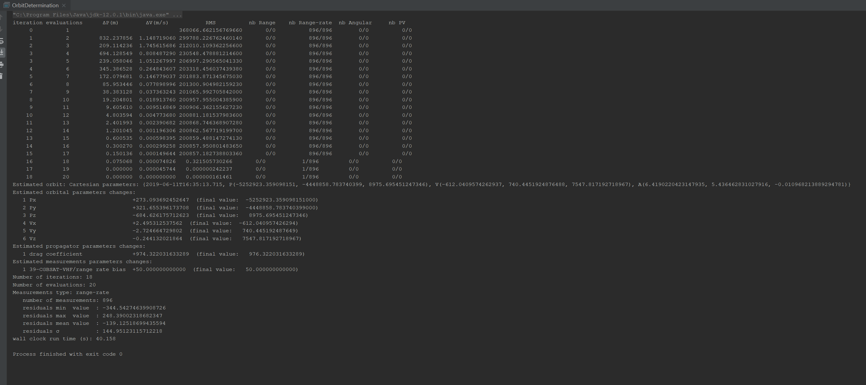
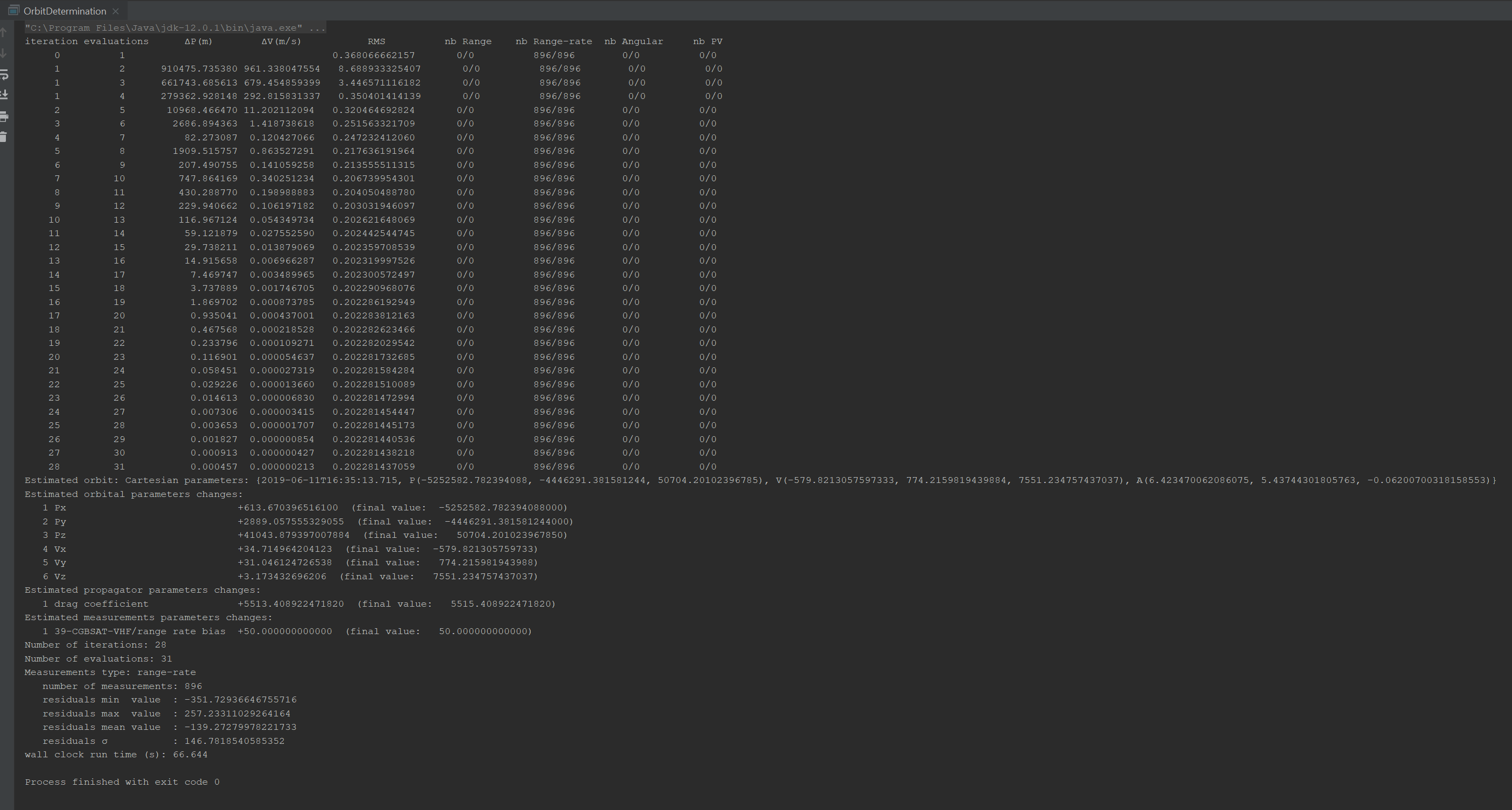
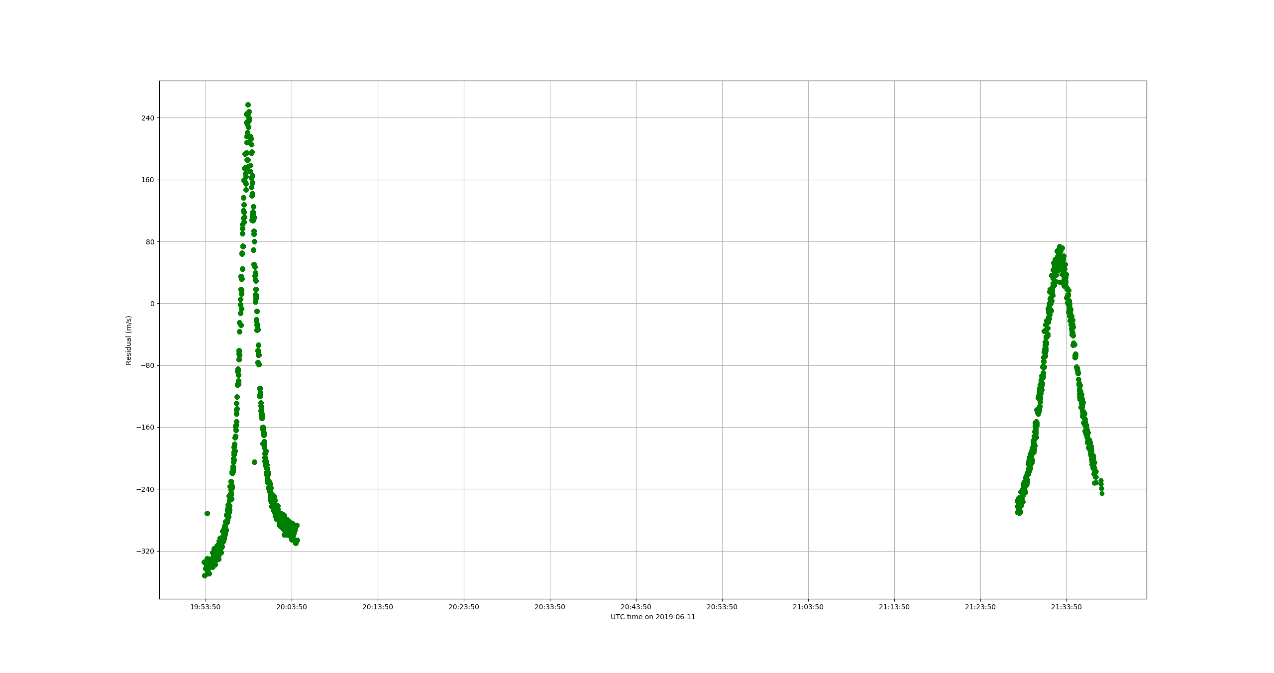
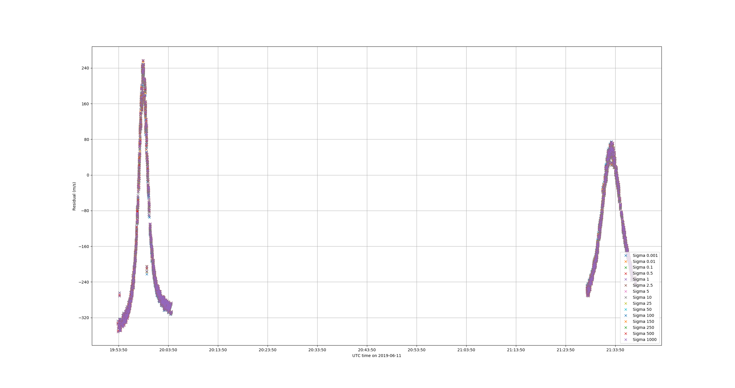
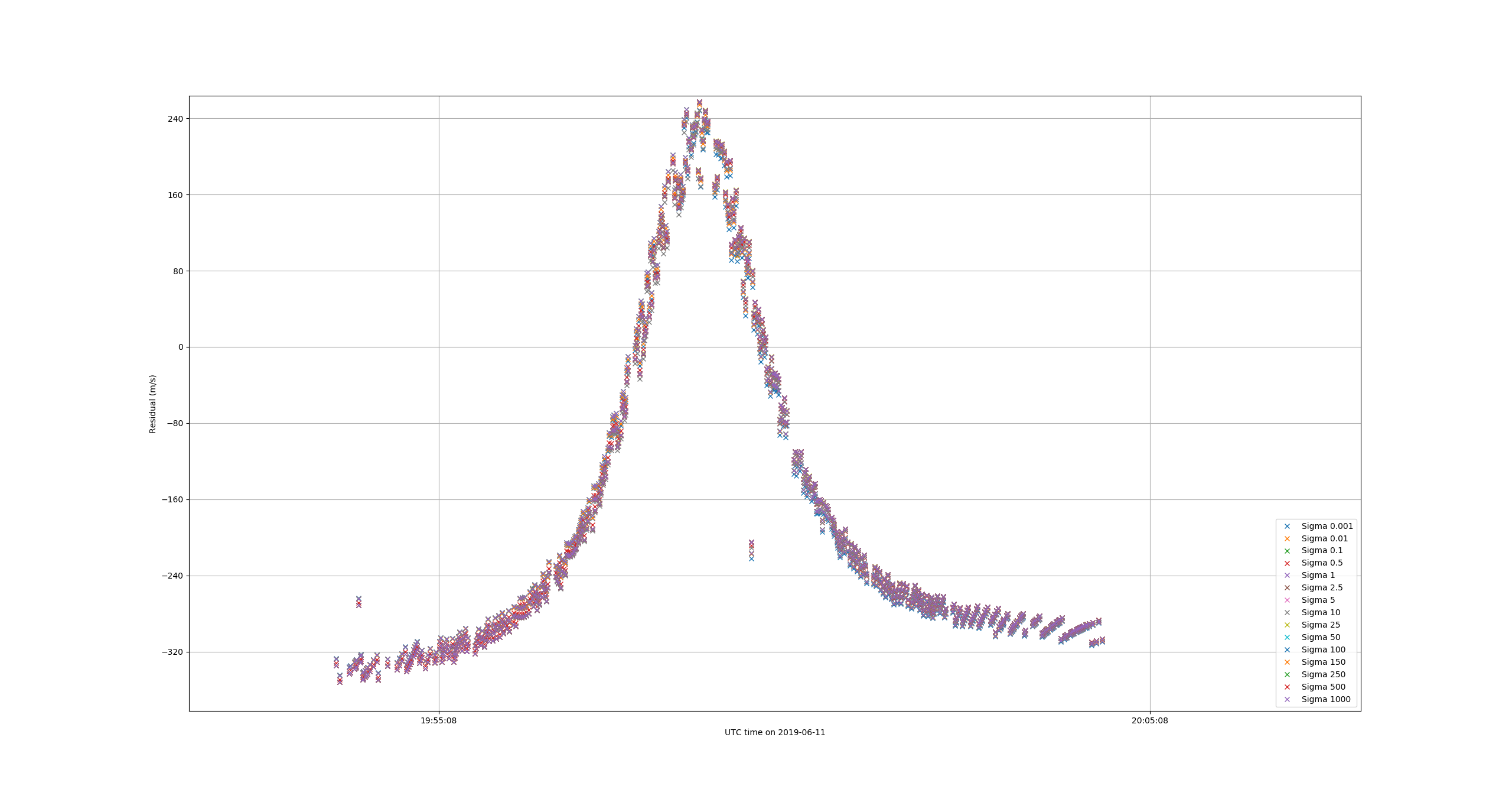
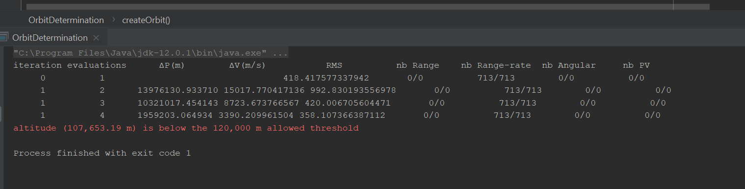
I think we are at the limit of what we can do with the current set of measurements. Playing around with the data seems to show that there are several different orbits/CD that are consistent with them. This means we have an observability problem and the various solutions are probably within a large covariance ellipsoid. Having only two passes one orbital period apart from each other and from one station only is not sufficient. The measurement noise of 15m/s is large. When we use Doppler measurements that are performed by dedicated equipment, the noise counts in centimeters or millimeters per second, not tens of meters. This was expected, as I said before, the shift we used were not designed for orbit determination.

One thing we could do is ask for more measurements. It would be nice to have several stations. Three or four stations, with as much passes over them as we can for a few orbits would be nice.

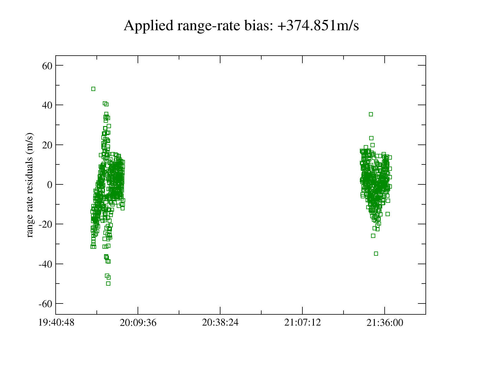
In the meantime, we can try to simulate this by ourselves, using the measurement generation feature. As the stations seem to have a large bias, we could generate our measurement sets with biases. This is done by adding another modifier to the RangeRateBuilder, either before or after having added the RangeRateTroposphericDelayModifier, as the order is irrelevant since both modifiers are additive:

  final double rangeRateBias = 375.0;
  builder.addModifier(new Bias<RangeRate>(new String[] { station.getBaseFrame().getName() + "-range-rate-bias" },
                                          new double[] { rangeRateBias },
                                          new double[] { 1.0 },
                                          new double[] { Double.NEGATIVE_INFINITY },
                                          new double[] { Double.POSITIVE_INFINITY }));

Of course, we should select a different, arbitrary, range-rate bias for each station as each one uses its own oscillator to generate or measure frequencies.

Concerning the model differences, I also suggest to change the measurement generator to use a numerical propagator with proper force models rather than a TLE to generate the measurements. This is done by creating the propagator first as follows:

  // atmosphere model for drag
  MarshallSolarActivityFutureEstimation msafe =
      new MarshallSolarActivityFutureEstimation(MarshallSolarActivityFutureEstimation.DEFAULT_SUPPORTED_NAMES,
                                                MarshallSolarActivityFutureEstimation.StrengthLevel.AVERAGE);
  manager.feed(msafe.getSupportedNames(), msafe);
  Atmosphere atmosphere = new DTM2000(msafe, CelestialBodyFactory.getSun(), earth);

  // this orbit is a dummy one, close to the first results from orbit determination from Max Valier satellite
  final NormalizedSphericalHarmonicsProvider gravity = GravityFieldFactory.getNormalizedProvider(12, 12);
  final AbsoluteDate             tOrb      = new AbsoluteDate("2019-06-11T16:35:29.149", utc);
  final TimeStampedPVCoordinates pvt       = new TimeStampedPVCoordinates(tOrb,
                                                                          new Vector3D(-5253194.0, -4400295.0, 80075.0),
                                                                          new Vector3D(-559.0, 764.0, 7585.0));
  final CartesianOrbit           orbit      = new CartesianOrbit(pvt, FramesFactory.getEME2000(), gravity.getMu());
  final OrbitType                type       = OrbitType.CARTESIAN;

  // set up numerical propagator
  final double[][]               tol        = NumericalPropagator.tolerances(10.0, orbit, type);
  final ODEIntegrator            integrator = new DormandPrince853Integrator(0.001, 300.0, tol[0], tol[1]);
  final NumericalPropagator      propagator = new NumericalPropagator(integrator);
  propagator.setOrbitType(type);

  // add a few realistic force models
  final double  cd          = 2.0;
  final double  area        = 0.25;
  propagator.addForceModel(new HolmesFeatherstoneAttractionModel(itrf, gravity));
  propagator.addForceModel(new ThirdBodyAttraction(CelestialBodyFactory.getSun()));
  propagator.addForceModel(new ThirdBodyAttraction(CelestialBodyFactory.getMoon()));
  propagator.addForceModel(new DragForce(atmosphere, new IsotropicDrag(cd, area)));

Then, we should replace the propagator used by the measurement generator to remove the TLE one and use the one we just created. This is done by replacing line

  final ObservableSatellite  os           = generator.addPropagator(TLEPropagator.selectExtrapolator(tle20190611));

by line

  final ObservableSatellite  os           = generator.addPropagator(propagator);

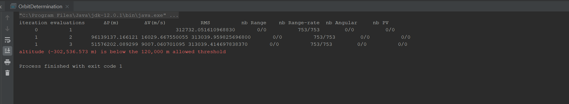
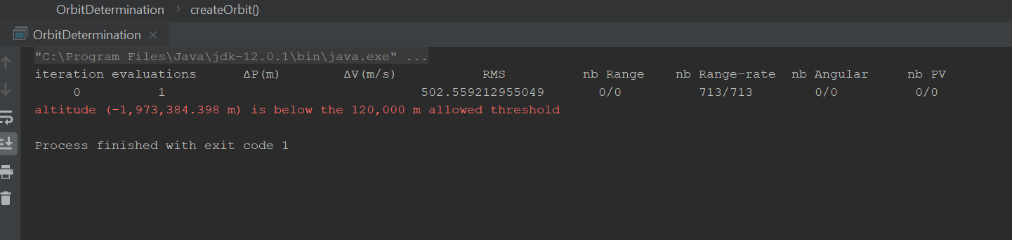
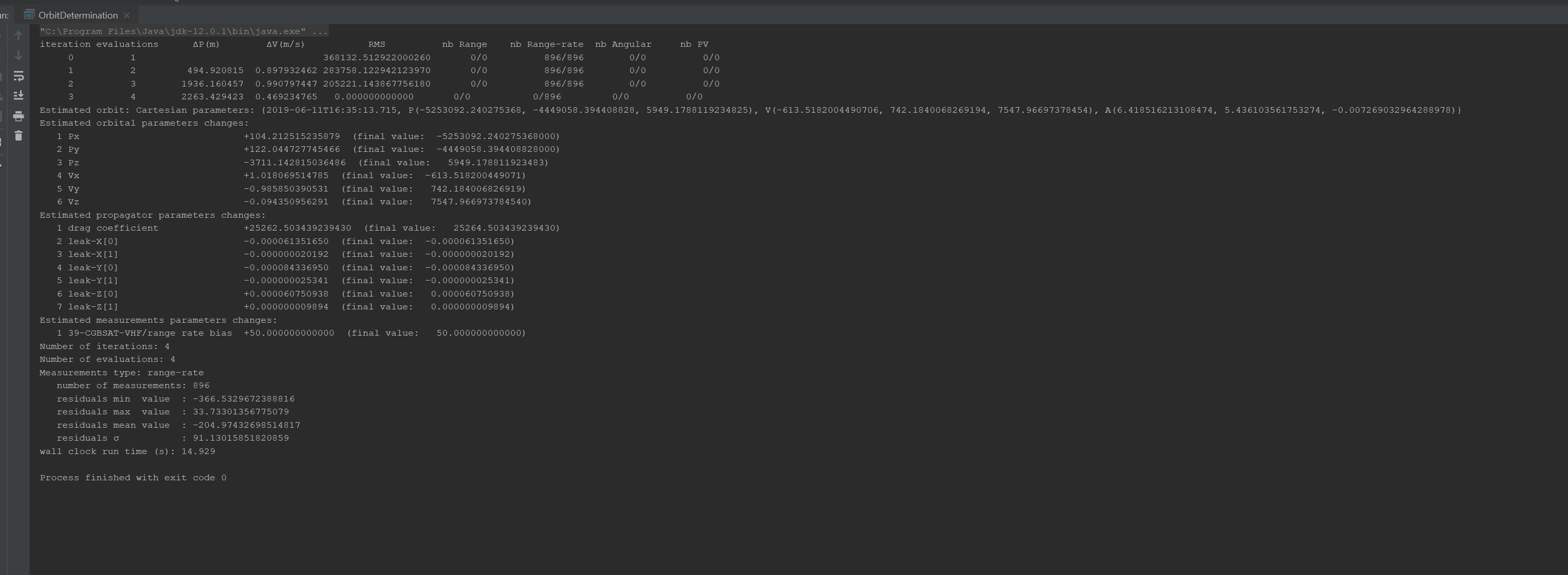
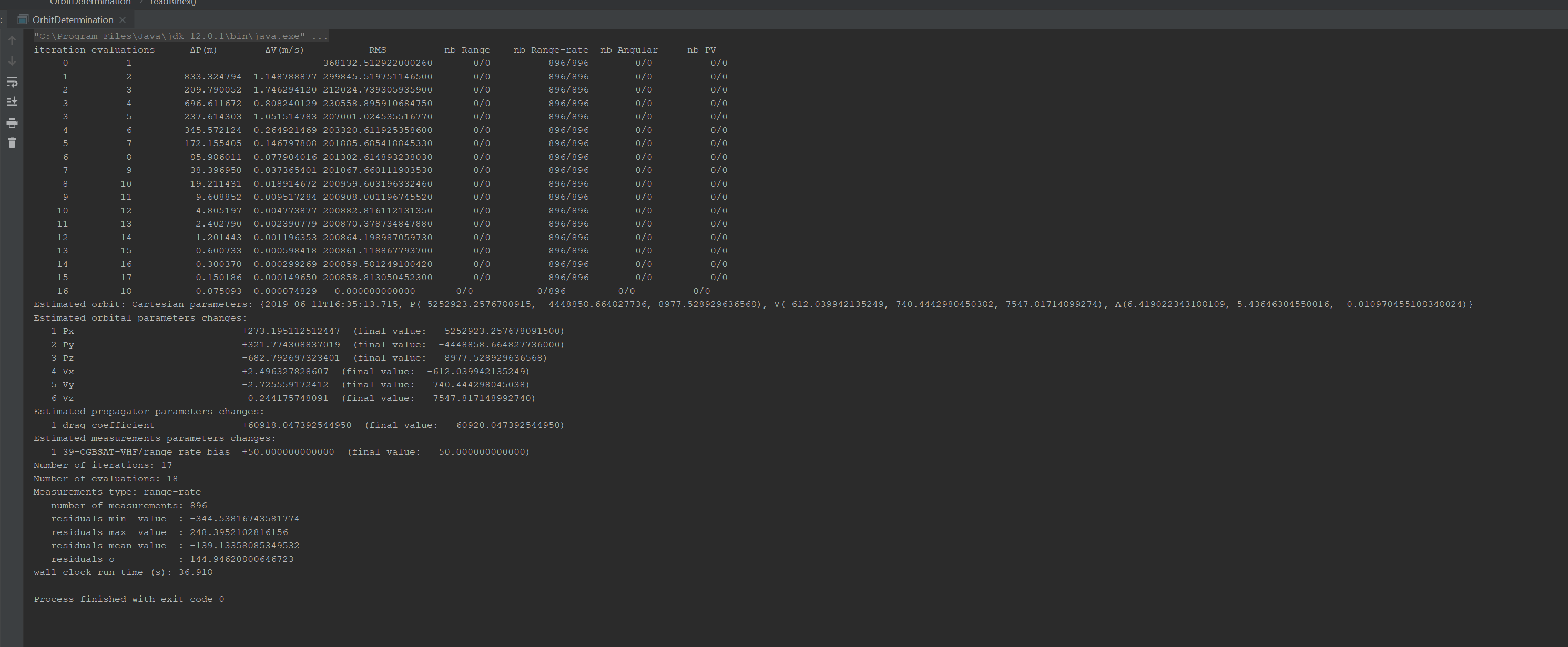
Could you do these changes, check everything works and commit the generator to the forge so it remains available for everyone to see? Then you can try to generate measurements on a made-up network, putting stations where you want and choosing a different bias for each station, and perhaps also change the drag coefficient from 2.0 to some other value, say 2.7 for example so we can see if the OD can recover it starting from its initial value of 2.0. Then you can pick up in the generated measurements all or only some passes as you want, playing with the configuration to see how it affects the results. Of course, if you have lots of stations, lots of passes, you should end up with a good orbit determination (you should get back the position-velocity that were hard-coded in the measurements generation program). What is interesting are the influence of number of stations, number of passes, time span over which OD is performed, biases, drag coefficient initial error…

Upon making those changes I got an error message of initial state not specified for orbit propagation when trying to run the measurement generation.
I managed to track the issue to the change to using the force models (it runs without issue if I use the TLEs instead.)
The range rate modifiers appear to work as intended. I have uploaded the current code to the forge.

I have spoken to Cees at SatNOGs regarding this, and he said he would look into if other stations could be used to generate Doppler curves (he’s altered his own using his software to be able to do this.) He has suggested using the Ephemer package for python to generate them otherwise.

Hi Noel, Luc,

I just caught up on this thread.

Just to fill you in; the data I provided is not generated from SatNOGS software. For my station I am using some of my own code to get timestamped waterfall plots. These are at a 1 second cadence and 10Hz (I recall) frequency resolution. For the MAX VALIER SAT data that I provided, the signal is CW (carrier wave or Morse code), and the data constains those frequency channels where the signal is highst in the spectrum.

There indeed will be an unknown frequency offset in the observations. This is because the receiver and also the transmitter are free running; both will have frequency offsets, of which we see the sum. This offset is also time dependent, so is likely to differ between different observations and also between different stations. You may get away with the assumption that the offset is constant during a 15 minute pass.

To improve the accuracy I may be able to run at higher time and frequency resolution.

Because the SatNOGS software at the moment does not provide timestamped waterfalls, it is not easy to provide data for multiple stations. A few other people are using my software and may be able to contribute, but it requires some organization on our part. Do you have an estimate what you would need?

1 Like

I see, sorry for that, my mistake. You need to add this line,for example after the call to propagator.setOrbitType(type):

propagator.setInitialState(new SpacecraftState(orbit,  16.0)); // the second argument is the spacecraft mass

Well, this is just what the measurement generator does, taking a lot of tiny effects into account (including EOP, tropospheric effects, time delay, biases…). I don’t know if the python package does the same and if its modelling is consistent with the one used in OD. As our OD is very close to the underlying physics, measurements must be either real measurements or measurements generated with a similar level of accuracy (definitely not a simple relative velocity projection).

I was suspecting that and wanted also to try estimating one bias per pass instead of one global bias. One way to do is easily right now would be to edit the files so the measurements from the second pass are considered to come from a second station. Changing the station name in the measurement file and adding a new station with this new name and at the same location as the first station would be enough. Then the two range-rate biases would be considered to be two different parameters and would be estimated independently to each other. It is good to know that the measurement is stable over one pass. If there was a regular change, like a linear drift, we could handle this too with a slight change in the code. I guess receiver temperature has an influence on frequencies stability isn’t it?

That would be great! Thanks a lot.

Unfortunately before we complete simulations, it would be difficult to give a detailed answer with the number of stations, how they are placed on the globe and what accuracy would be needed. So here are only some hints:

  • it would be nice to have stations widespread on the globe to spread observation points on the orbit
  • it would be nice to have observations on a time span over 3 or 4 orbital periods
    (this would probably help with the drag coefficient which is totally unrealistic for now)
  • it would be nice to have a couple of stations that could see the satellite at the same time to
    get rid of some possible biases (say stations a few hundreds of kilometers away from each other)
  • if possible, the stations should be as accurately synchronized with UTC as possible (using NTP
    or a local GNSS receiver providing a pulse per second signal)
  • of course, all the measurements should be one the same satellite and for the same orbits, so I
    agree this needs some synchronization among the network
  • we would also like to know if people contributing these measurements (including yourself) would
    agree to be credited for this in the final project report (and maybe in a following conference paper…)

Perfect thanks. The generated measurement program now runs without error.
Unfortunately though the orbit determination program crashes when I run the generated files with the following outputs before failing

Do you think this is due to something that I need to alter in the maxvalier.in file or is it something that I need to change in the generator? (I have attached the generated measurements for reference)

generated-doppler-39-CGBSAT-VHF.dat (46.3 KB)

I had a feeling this might have been the case. That makes sense regarding the required level of accuracy, I hadn’t considered that as an issue :sweat_smile:.

I could tune this quite easily in the measurement converter that I wrote, so that it has different stations ID’s for each pass.

Hi @cgbsat,
I’ve seen on the SatNOGS website that you appear to have a UHF antenna as well as a VHF one, is that correct?
If so are you able to run your own software in the UHF frequency range?

Thanks,
Noël

You should try to comment out the orbit_tle_line_1 and orbit_tle_line_2 keys in maxvalier.in and
uncomment lines orbit.date and orbit.cartesian.{px, py, pz, vx, vy, vz}. The date should be set to 2019-06-11T16:35:29.149 and the Cartesian coordinates should be set to values close (but not equal) to the coordinates used in the measurements generation. I would suggest changing the position a few tens of kilometers and the velocity a few tens of meters/second (for reasons of consistency due to energy, variations in position and variations in velocity are roughly different by a factor 1000, hence the values I suggest).

The reason to set up an initial orbit in the maxvalier.in file close but not similar to the one used for measurment generation is to see if orbit determination does its job. It should find that the initial orbit is slightly wrong and correct it, to come back to the one that was used for generation.

Thanks for those corrections.
I ran the orbit determination with the following settings on date and p-v in the maxvalier.in file:
orbit.date = 2019-06-11T16:35:29.149
orbit.cartesian.px = -5273194
orbit.cartesian.py = -4450295
orbit.cartesian.pz = 110075
orbit.cartesian.vx = -585
orbit.cartesian.vy = 790
orbit.cartesian.vz = 7610
and drag.cd.estimated = false

The px,py,pz coordinates correspond to an orbital position of 503.4km and vx,vy,vz correspond to an orbital velocity of 7673m/s (compared to the 475km and 7643m/s used in the generator program.)

When run through the orbit determination program it yielded enormous residuals (up to 7million) and an orbital altitude of that appeared much too large. Upon some investigation I found that the generated measurements were in m/s rather than the km/s used by the orbit determination program, so I changed this to the correct units.

Upon running it again, with no other changes, I got the same error as before (although with smaller RMS values, so that’s something):

I have tried to alter the orbital parameters to: px = -5423194 , py = -4550295 , pz = 250075 , vx = -735 , vy = 740 , vz = 7760, but got the same error:

I have attached the generated files for the initial run with doppler measurements in m/s.
orbit-determination-range-rate-residuals-generated.out (79.7 KB)
orbit-determination-log-generated.out (5.1 KB)

The error about altitude below 120km is related to the atmosphere model used for drag force computation. The orbit determination tutorial has been set up using the DTM2000 model which does not extends down to ground. Such types of limitations are frequent in atmosphere models, as they are intended for satellites. At 120km, you are already very low, at reentry level. We could use another atmosphere model (and in fact a much better one as DTM2000 is really not recommended anymore). The NRLMSISE2000 model is now the one we recommend, and it has the additional benefit of extending down to ground.

This, however, is only a sign of something else wreaking havoc: we should not go from 500km to 120km with a “normal” drag coefficient and no maneuver. In fact, the OD process get lost right at the beginning. Looking at your first iteration, it tries to move the satellite by almost 14000km. This can be avoided by reducing the initial step bound factor (parameter estimator.Levenberg.Marquardt.initial.step.bound.factor). This parameter has some black magic included: there are no perfect rules to set it, its mostly trial and error. When close to Earth, as atmosphere density changes exponentially, some test orbits the optimizer wants to evaluate may end up triggering the exception you have seen, so we try to prevent it testing orbits too far, even if it implies doing more iterations. The second attempt with vx set to -735 is clearly already too far, 160m/s difference with the real orbit is a tremendous initial error.

So I tried with this:

orbit.date = 2019-06-11T16:35:29.149
orbit.cartesian.px = -5273194
orbit.cartesian.py = -4450295
orbit.cartesian.pz = 110075
orbit.cartesian.vx = -585
orbit.cartesian.vy =  790
orbit.cartesian.vz = 7610
...
estimator.Levenberg.Marquardt.initial.step.bound.factor = 100.0

Then the process converges with the following results:

iteration evaluations      ΔP(m)        ΔV(m/s)           RMS          nb Range    nb Range-rate  nb Angular     nb PV
     0          1                                 502.559212955049       0/0          713/713        0/0          0/0   
     1          2       41897.042311  5.372745063 498.755565145088       0/0          713/713        0/0          0/0   
     2          3       76995.153909 11.272244311 491.320402999840       0/0          713/713        0/0          0/0   
     3          4      104784.168766 24.667473984 477.497649253095       0/0          713/713        0/0          0/0   
     4          5       53358.435567 51.472432766 442.321488682624       0/0          713/713        0/0          0/0   
     5          6       12346.634942 78.272402581 309.656257555581       0/0          713/713        0/0          0/0   
     6          7       10743.579822 92.299454042  85.332350236302       0/0          713/713        0/0          0/0   
     7          8      171563.213336 170.204556144  63.152158757981       0/0          713/713        0/0          0/0   
     8          9       60045.019913 178.367553223  34.203601645514       0/0          713/713        0/0          0/0   
     9         10       75703.814940 61.910993424   9.203202160007       0/0          713/713        0/0          0/0   
    10         11       12612.507287 25.106258191   1.093589206022       0/0          713/713        0/0          0/0   
    11         12         456.426950  1.202983056   1.049911494077       0/0          713/713        0/0          0/0   
    12         13           1.698701  0.001659690   1.049911167960       0/0          713/713        0/0          0/0   
    13         14           0.002574  0.000002804   1.049911167960       0/0          713/713        0/0          0/0   
Estimated orbit: Cartesian parameters: {2019-06-11T16:35:29.149, P(-5253009.438816775, -4400520.679405428, 80427.86229386796), V(-558.9409310057042, 764.267511436562, 7584.967970138002), A(6.505523654578354, 5.449769642672016, -0.09960487730587128)}
Estimated orbital parameters changes: 
   1 Px                             +20184.561183225363  (final value:  -5253009.438816775000)
   2 Py                             +49774.320594572460  (final value:  -4400520.679405428000)
   3 Pz                             -29647.137706132038  (final value:   80427.862293867960)
   4 Vx                             +26.059068994296  (final value:  -558.940931005704)
   5 Vy                             -25.732488563438  (final value:   764.267511436562)
   6 Vz                             -25.032029861998  (final value:   7584.967970138002)
Estimated propagator parameters changes: 
Estimated measurements parameters changes: 
   1 39-CGBSAT-VHF/range rate bias  -0.009368765028  (final value:   374.990631234972)
Number of iterations: 13
Number of evaluations: 14
Measurements type: range-rate
   number of measurements: 713
   residuals min  value  : -48.68390007557355
   residuals max  value  : 45.32828574650921
   residuals mean value  : -2.8188214470925566E-9
   residuals σ           : 15.75972309642003
wall clock run time (s): 80.059

This is much better than earlier, but the Doppler noise prevents getting a good orbit. We are at 457m in position.

We estimated the range rate bias at almost 0, though, there is perhaps a problem there, it should be estimated at 375m/s as it is what is configured in the generation program. Did you remove the bieas before generating the data?

We are improving, though.