Unexpected results in basic propagations due to normalized gravity provider

ShikaDing · January 17, 2021, 3:09pm

Hello!

I’m new to OREKIT and the forum and just getting my feet wet with some basic scripts. Moving beyond the tutorials, I’ve been getting some results I cannot understand which I’ve isolated due to the effect of the normalized gravity provider I’ve pulled from a tutorial, and the max degree/max order used when called.

I’m using a python script with the python wrapper, and the basic task I was trying to test was tracking satellite separation over time for two satellites in a single plane separated by some initial true anomaly (approx circular orbits, ~1000km altitude).

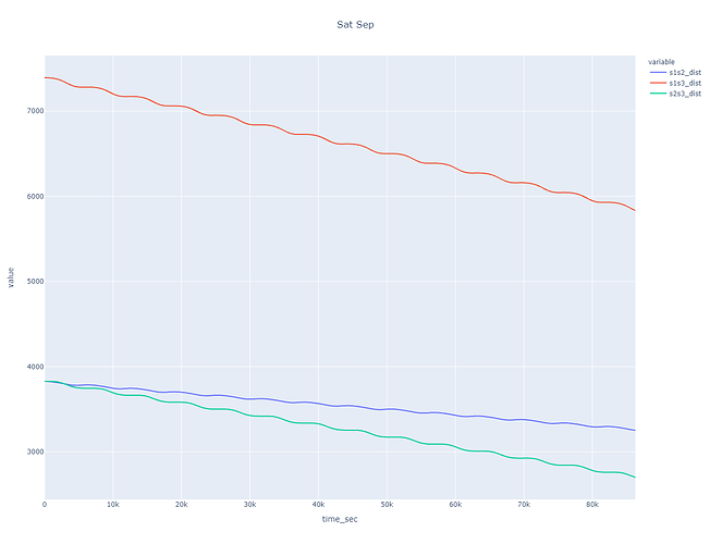
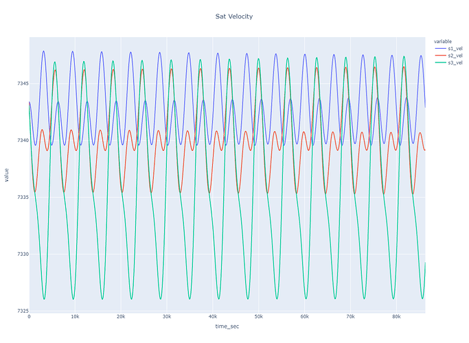
The odd behavior itself is how the sat separation decreases VERY QUICKLY, visible in the plot of sat separations, as well as velocities (plots attached).

Having a hard time believing this a correct astrodynamical effect, so I tested several things and found that if I change the gravity provider from:
gravityProvider = GravityFieldFactory.getNormalizedProvider(8, 8)
to:
gravityProvider = GravityFieldFactory.getNormalizedProvider(1, 1)

… the separation is much more constant with time. This separation drift is also a function of inclination, larger the inclination, larger the effect, but behaves roughly as expected with i < 10 deg

Other ways I’ve tested this and seen the same effect:

numerical and analytic propagators
Keplerian and Equinoctial orbit types (all ~1000km altitude)
Inclinations 0…100, higher inclination, more exaggerated the effect

So I understand the gravity provider as accounting for asymmetries in earth’s field due to mass distributions, but this effect just seems hyper-exaggerated. Does anyone have any insight into this and how to properly do high precision LEO orbit propagations?

Simplified code is below for reference.

Thank you!

'''Set up small number of satellites in ONE constellation plane, and analyze how their separation changes
over time'''

import orekit
from orekit.pyhelpers import setup_orekit_curdir
from orekit import JArray_double
from org.orekit.bodies import  OneAxisEllipsoid
from org.orekit.frames import  FramesFactory
from org.orekit.time import TimeScalesFactory, AbsoluteDate
from org.orekit.orbits import KeplerianOrbit, OrbitType, EquinoctialOrbit
from org.orekit.propagation.analytical import KeplerianPropagator, EcksteinHechlerPropagator
from org.orekit.utils import Constants
from org.orekit.propagation import SpacecraftState
from org.orekit.orbits import OrbitType, PositionAngle
from org.orekit.propagation.numerical import NumericalPropagator
from org.hipparchus.ode.nonstiff import DormandPrince853Integrator
from org.orekit.forces.gravity.potential import GravityFieldFactory
from org.orekit.forces.gravity import HolmesFeatherstoneAttractionModel
from org.orekit.utils import IERSConventions

import numpy as np
import pandas as pd
import plotly.express as px
from math import radians, degrees, sin, cos, tan

vm = orekit.initVM()
setup_orekit_curdir()

# Set propagator type:
analytic = True

# Times:
# - Overall duration in seconds for extrapolation
duration = 3600 * 24 * 1.0  # hr * 24 * days
step_time = 60.0 * 2

# - Time array in orekit AbsoluteDate format
utc = TimeScalesFactory.getUTC()
startDate = AbsoluteDate(2021, 1, 16, 11, 0, 00.000, utc)
t_arr = [startDate.shiftedBy(float(dt)) for dt in np.arange(0, duration, step_time)]    # list of AbsoluteDate objects
t_arr_sec = [i * step_time for i in range(len(t_arr))]                 # list of ints

# Some Constants
ae = Constants.WGS84_EARTH_EQUATORIAL_RADIUS
mu = Constants.WGS84_EARTH_MU
initialStates = []  # holds sat initial states
prop_list = []      # holds a propagator for each orbit (same prop, diff orbit)
sat_pos = []  # holds lists of Vector3D types for each satellite for each timestamp. Each entry holds every time
sat_vel = []

# Set up Satellites data
# - Polar plane example:
planes = 1
sats = 3

# Equinoctial Orbit elements, common across satellites in-plane:
a = ae + (1000.0 * 1015)        # SMA, meters
e_e = 0.0001
i = 99.0                        # inclination
raan = radians(0.0)             # right ascension of ascending node, rads
#lv = v + ω + Ω                 # anomaly, see below
#  ω is the argument of perigee, Ω is right ascension of ascending node, M is mean anomaly,
#  E is eccentric anomaly and υ is true anomaly
dAnom = 30.0                    # in plane spacing, true anomaly delta
satellite_mass = 100.0          # kg

# Inertial frame where the satellite is defined
inertialFrame = FramesFactory.getEME2000()

# Set up each orbit state:
for sat in range(sats):
    omega = radians(0.0)            # perigee argument (pa in Orbit class), rads. TA and MA defined wrt this
    raan = radians(0.0)             # right ascension of ascending node, rads
    t_anom = radians(sat*dAnom)     # True anomaly, rads

    ex = e_e * cos(omega + raan)
    ey = e_e * sin(omega + raan)
    hx = tan(i / 2) * cos(raan)
    hy = tan(i / 2) * sin(raan)
    Lv = t_anom + raan + omega      # true longitude argument
    equinoc_initialOrbit = EquinoctialOrbit(a,
                                            ex,
                                            ey,
                                            hx,
                                            hy,
                                            Lv,
                                            PositionAngle.TRUE,
                                            inertialFrame, startDate, mu)
    initialOrbit = equinoc_initialOrbit

    # Make list of initial states, and list of propagators tied 1:1 to each state
    initialStates.append(SpacecraftState(initialOrbit, satellite_mass))
#print(*initialStates, sep='\n')

# Propagators:
''' For the numeric propagator to make sense it needs some forces acting on the satellite. Here we are adding a gravity 
field model.For a more detailed propagation, other force models can be added.'''
itrf = FramesFactory.getITRF(IERSConventions.IERS_2010, True)   # International Terrestrial Reference Frame, earth fixed
earth = OneAxisEllipsoid(Constants.WGS84_EARTH_EQUATORIAL_RADIUS,
                         Constants.WGS84_EARTH_FLATTENING,
                         itrf)
gravityProvider = GravityFieldFactory.getNormalizedProvider(8, 8)
#gravityProvider = GravityFieldFactory.getNormalizedProvider(2, 2)   # max degree, max order from first supported file


if analytic:
    # - Note on EckStein Hechler: It is adapted to nearly circular orbits (eccentricity less than 0.05 and at most 0.1)
    # ..and does not work for inclinations close to the critical inclinations (~63.43 deg and ~116.57 deg).
    # but EH is also NOT good for very small eccentricities, ~ < e-5. Usable range is 1e-5 < e < 0.1
    # - Other analytic options: J2Differential, KeplerianPropagator
    for state in initialStates:
        pos = []
        vel = []

        # Choose one propagator:
        propagator = EcksteinHechlerPropagator(state.getOrbit(),
                                               Constants.EIGEN5C_EARTH_EQUATORIAL_RADIUS,
                                               Constants.EIGEN5C_EARTH_MU, Constants.EIGEN5C_EARTH_C20,
                                               Constants.EIGEN5C_EARTH_C30, Constants.EIGEN5C_EARTH_C40,
                                               Constants.EIGEN5C_EARTH_C50, Constants.EIGEN5C_EARTH_C60)
        # propagator = KeplerianPropagator(state.getOrbit())

        # Propagate: prototype is propagate(start,end)
        #sat_pos = [propagator.propagate(startDate, t).getPVCoordinates().getPosition() for t in t_arr]
        #sat-vel = [propagator.propagate(startDate, t).getPVCoordinates().getVelocity() for t in t_arr]
        for t in t_arr:
            p_state = propagator.propagate(startDate, t).getPVCoordinates()
            pos.append(p_state.getPosition())
            vel.append(p_state.getVelocity())
        sat_pos.append(pos)
        sat_vel.append(vel)

# Calculate separations:
s1s2_dist = [i[0].distance(i[1]) for i in list(zip(sat_pos[0], sat_pos[1]))]
s1s3_dist = [i[0].distance(i[1]) for i in list(zip(sat_pos[0], sat_pos[2]))]
s2s3_dist = [i[0].distance(i[1]) for i in list(zip(sat_pos[1], sat_pos[2]))]

# Calculate velocities:
s1_vel = [v.getNorm() for v in sat_vel[0]]
s2_vel = [v.getNorm() for v in sat_vel[1]]
s3_vel = [v.getNorm() for v in sat_vel[2]]

# Convert to km for plotting:
s1s2_dist = np.divide(s1s2_dist, 1000)
s1s3_dist = np.divide(s1s3_dist, 1000)
s2s3_dist = np.divide(s2s3_dist, 1000)

# Set up df for plotting:
df = pd.DataFrame(data=zip(t_arr_sec, s1s2_dist, s1s3_dist, s2s3_dist,
                           s1_vel, s2_vel, s3_vel),
                  columns=['time_sec', 's1s2_dist', 's1s3_dist', 's2s3_dist',
                           's1_vel', 's2_vel', 's3_vel'])

fig = px.line(df, x='time_sec', y=['s1s2_dist', 's1s3_dist', 's2s3_dist'],
              title='Sat Sep')
fig.update_layout(title_x=0.5)
fig.show()

fig = px.line(df, x='time_sec', y=['s1_vel', 's2_vel', 's3_vel'],
              title='Sat Velocity')
fig.update_layout(title_x=0.5)
fig.show()

### Note: Nominal sat-sep, based on isosceles triangle:
# - r =  6379 + 1015 = 7394
# - base angle = theta = 180 - 27.692/2 - 90 = 76.154
# - base = 2*r*cos(theta) = 3,538 km
# - Sep between adjacent polar sats is 3,538 km

ShikaDing · January 18, 2021, 3:56pm

Not sure how to edit original post - but in the simplified code example it doesn’t even implement the gravity provider but gets the same effect due to the EcksteinHechlerPropagator with spherical harmonics.

So there’s two ways (at least) to reproduce this behavior:

analytic propagation with EcksteinHechlerPropagator
numeric propagation with gravity provider and it’s specified degree/orders

Expected behavior comes from using the simple Keplerian propagator, the velocities of each satellite varies around the orbit, but are identical to each other with a phase shift (see below). Why do the more ‘accurate’ gravity models act this way (original post)? It seems too extreme.

luc · January 21, 2021, 8:14am

Hi, and welcome to the forum and to the Orekit community.

I think the behavior you observe is correct and related to osculating vs. mean parameters differences.

When you set up the orbits, they all start from same semi-major axis and eccentricity, and the anomaly is spread every 30 degrees. Then you start a numerical propagator that considers that the orbit is given in osculating parameters. Osculating parameters and zonal perturbations generates periodic effect on the semi-major axis and eccentricity. For semi major axis, you could say we have something like:

  a_osc = a_moy + f(anomaly)

but as you use the same a_osc for all satellites, this implies you really use

  a_moy_i = a_osc - f(anom_i)

hence you have a different mean semi major axis. IMHO, it should explain the observed drift.

ShikaDing · January 21, 2021, 6:28pm

Hi Luc,
Thanks for the reply, and I think you’re right. My investigations in the meantime have come to the same conclusions, that even with such small eccentricities, the osculating SMA varies enough that this seeding method is not really putting the satellites on the same orbits to retrace each other’s tracks.

I also tested a seeding method of starting with just one satellite, then propagating it to the second position in the plane, resetting that state’s date to the beginning, and looping over that up to n-sats. That took care of all the osculating elements to get close to identical orbits for satellites phased in a plane.

How realistic that approach is might be another question, but it sure helped get things rolling with Orekit!

Cheers

luc · January 22, 2021, 10:00am

Another method you could try is to set up your orbits just as you did before, with regular
distribution of anomalies and all other parameters kept identical, and to use DSSTPropagator.computeOsculatingState() with the force models you want to convert these
orbits into osculating orbits before setting the propagators.

The DSST model will take care to add the correct short periodic terms for you so the osculating propagator will behave properly, but by definition all your orbits will have the same mean semi major axis.

ShikaDing · January 22, 2021, 3:11pm

Interesting, thanks for the suggestion. I actually just stumbled upon the DSSTPropagators while trying to extract mean orbit elements from this model, so just learning about that in general. I’m not familiar with what that is really, so something new to read up on!

ShikaDing · January 26, 2021, 4:17pm

Luc, if you happen to see this I tried out what you suggested, but found that the input mean-state and output osculating state were identical, maybe I misunderstood what you mean.

My approach was to:

set up a DDSTPropagator with same integrator from sample above (DormandPrince853):
DSSTPropagator(integrator, PropagationType.MEAN)
add force model (tried most of them, eg. Newtonian, zonal, tesseral)
convert the input mean state (the ones with staggered anomalies) into osculating states, via DSSTPropagator.computeOsculatingState(state, att, force_model_collection). The output of this is identical to ‘state’.
Feed osculating state into numerical propagator loop to generate time-series data

The result is orbits that look like the ones in the initial post, with slightly different mean SMAs, periods, etc., and quickly diverging separations So I think I’m not implementing the idea correclty. Is there some other step you have in mind?

Thanks!

luc · January 26, 2021, 4:59pm

Note that the integrator for DSST should be set up with a much longer step size than numerical propagator. As the integrator is used only for mean elements that vary very slowly, the step size is often set to a few orbits or even one day depending on orbit!

This is however not useful here because you should not set up a DSST propagator at all, you should only use the static method, but I don’t know how it works from Python. In Java, you just call DSSTPropagator.computeOsculatingState(state, attProvider, forces) using the name of the class DSSTPropagator and not a reference to some instance.

ShikaDing · January 29, 2021, 7:35pm

I see, thanks for that info on the DSST setup in general, and in this case that certainly simplifies things.

In python the call looks the exact same (java methods are wrapped to make it so). For a while I was having trouble understanding the correct usage of the third argument to .computeOsculatingState(), the ‘Collections<DSSTForceModel> force’ as it’s defined, and that was mistakenly setting the ‘forces’ to Null.

If it helps anyone in the future, here’s how I got it to work:
Casting DSSTForceModel interface type to the correct Collections type for method call, then the method call itself:

force_model_collection = ArrayList().of_(DSSTForceModel)

Then add forces to this collection variable, eg:

force_model_collection.add(DSSTNewtonianAttraction(mu))

And finally:

osc_state = DSSTPropagator.computeOsculatingState(state, att, force_model_collection)