Hi all,
I am new to Orekit and trying to use it in Matlab.
My goal is to create two orbits that are equal to within a few centimeters. One of the orbits will be the basis for a later simulation and the other will then be used to evaluate the simulation (with a small difference, to make the procedure more realistic). My procedure is as follows.
I simulate an orbit for one day. From this I create a PV object every 30 seconds.
I take this PV object as observations for a BatchLSEstimator object.
The InitialOrbit for simulation and adjustment is the same.
As integrator I take the ClassicalRungeKuttaIntegrator for simulation and adjustment, in each case with the same step size. As propagator I use the NumericalPropagator for the simulation and the adjustment.
In a first test, I want to see if the estimated orbit is the same as the simulation orbit.
With an integrator step size of 1 second, the difference between both orbits is zero. But if I increase the integrator step size, the errors become bigger and bigger.
I would think that it makes no difference how large the step size becomes, as long as it is the same in simulation and adjustment.
Does anyone perhaps have a tip for me where this behaviour is coming from?
Also, the reference frames (EME2000) are always the same. I am also using the newest Orekit version (11.1) and Matlab 2020a. And for the first test, i do not add forcemodels.
Later I would like to introduce different atmospheric models for simulation and adjustment to create a difference in the orbits.
As the second orbit is adjusted from a sampled points, it will not be the same as the original orbit. You will always get some numerical noise. You should also note that ClassicalRungeKuttaIntegrator is a very crude integrator. As it is very low order (4), it needs short time steps (one second is indeed very small) but smal time steps induce lots of numerical noise. I would suggest to use a much more efficient and accurate integrator, typically DormandPrince853, with tolerances set to say 0.001m.
When you write the errors become bigger and bigger, how does it increase? Are you at centimeter, meter, or kilometer order of magnitude after one day?
Also how are the PV created? Are they directly generated from one propagation and provided to the second one in the same program or are the coordinates written to an intermediate file and then parsed for adjustment?
Hi @luc,
thanks for your fast reply.
Yes, RungeKutta is not the best Integrator, but I thought in my case ok, because i only want orbits for simulation purposes. I only was wondering that my orbit difference is complete zero if i run my code with RungeKutta stepsize 1 sec and in submeter level if change the stepsize to 30 seconds.
Now, I followed your tip and tried the DormandPrince 8 (5,3) Integrator instead. With this integrator (minStepSize: 0.001, maxStepSize: 300, positionError: 0.001) i have a difference of 1e-8 m, but not zero like in the RungeKutta (stepSize: 1 sec) case.
I simulate and estimate in the same script. So i propagate an orbit and save the position/velocity directly in a PV object.
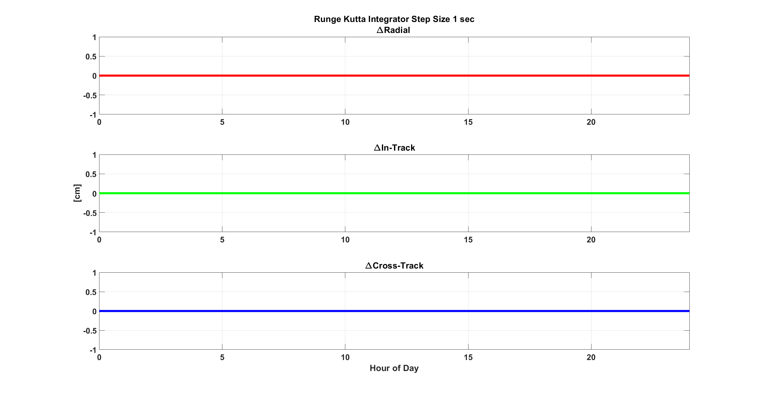
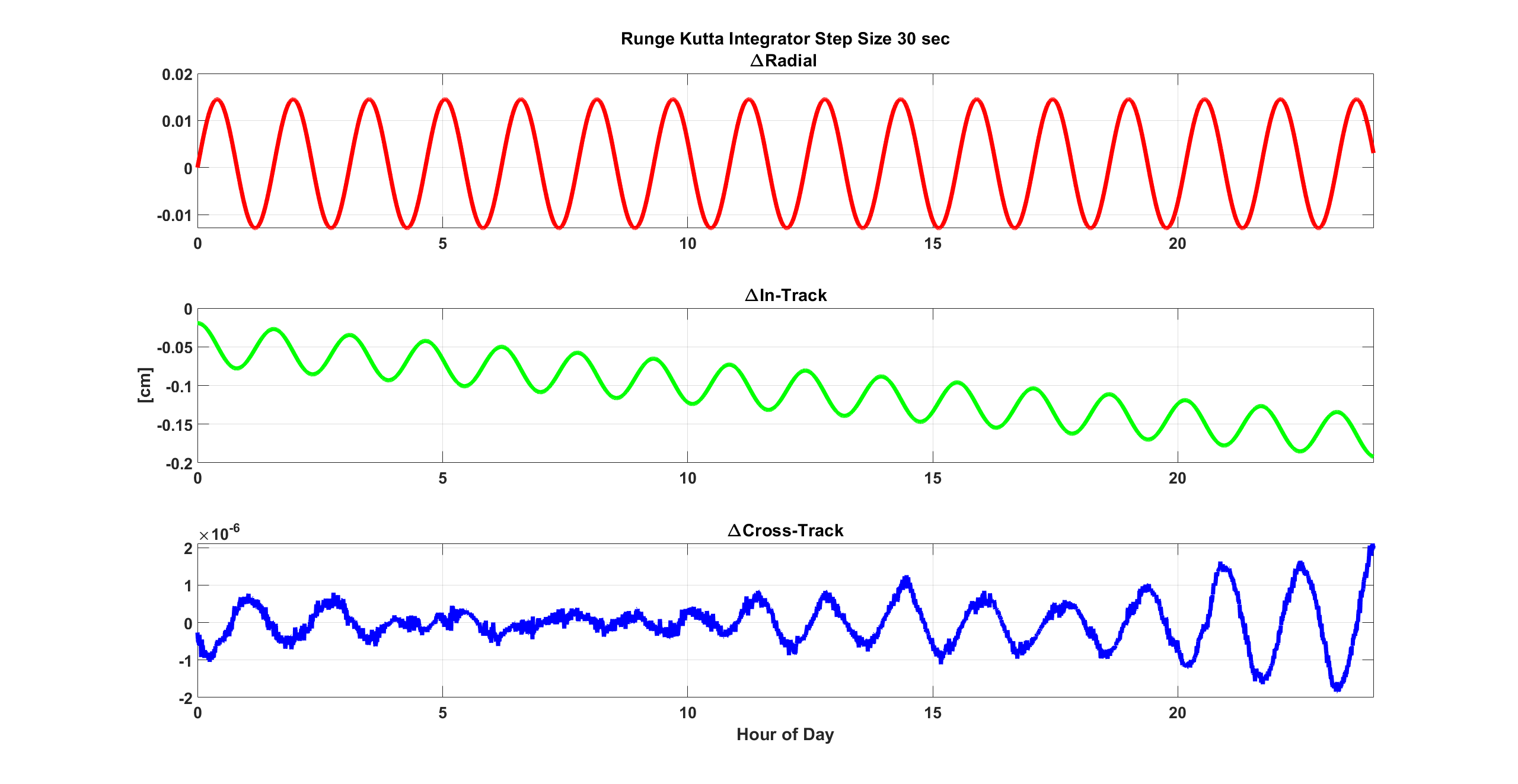
And to explain the meaning of “errors become bigger and bigger” i attached two figures.
In the figures you see the difference between the two orbits in radial, in-track and cross-track. Units are centimeter. One figure with an integrator step size of 1 sec and the other one with an integrator stepsize of 30 sec.
In principal the differences with the DormandPrince853 Integrator are very small and can be neglected for my simulation. I only was confused that it is possible to get a different difference by only changing the step-size.
A possible explanation (just a wild guess from me), is that when using BatchLSEstimator, the estimator will need to get the state at the measurement date, which may be different from the exact steps boundaries. For this, it uses the dedicated interpolator provided by each integrator. The interpolator always has a lower order than the integrator. The reason for that is that the integrators coefficients (the elements in the Butcher’s arrays that define the integrator) are the solutions of so-called order conditions at the step endpoints. So the error collapses are the end of the steps, but as the order conditions cannot all be met inside the step, the interpolator is at least one order less. As a result, interpolated points may be off by a little bit.
I am in fact surprised that you get exactly zero with 1s step size and classical Runge-Kutta. Perhaps this is a lucky situation in which every PV is produced exactly at a step boundary.