Hello again, sorry for the late reply
I did try what you suggested, interestingly enough, if I compare the equinoctial elements of the two states they do indeed match.
However, once again, if I try to convert the orbit to a Keplerian one, or if I use the getI() method of SpacecraftState, the inclination doesn’t match.
I obtain the same result if I use Hx and Hy to manually compute the inclination. I have literally no clue as to what’s wrong.
Are you using mean elements in your conversion?
If so, then I believe that is the problem. The “average” property is bound to the type of coordinates. So if you convert them in another system, you introduce an error. I think we can summarize this by “non linear maps and integrals are not interchangeable”. This is why comparing Cartesian parameters showed a discrepancy.
Yes, what I meant before was that I was converting the mean equinoctial elements to Keplerian ones.
I’m not very familiar with the DSST theory, but, given your answer, I get that mean Keplerian elements don’t really exist and the nomenclature of “mean elements” is strictly bounded to the equinoctial elements. Is that correct?
That’s very weird indeed…
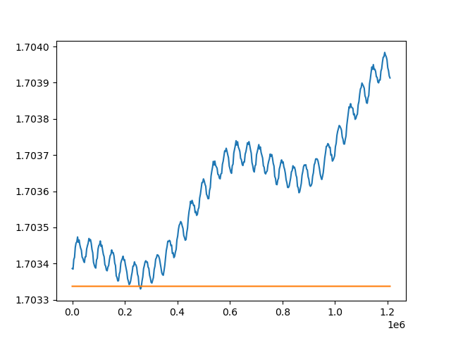
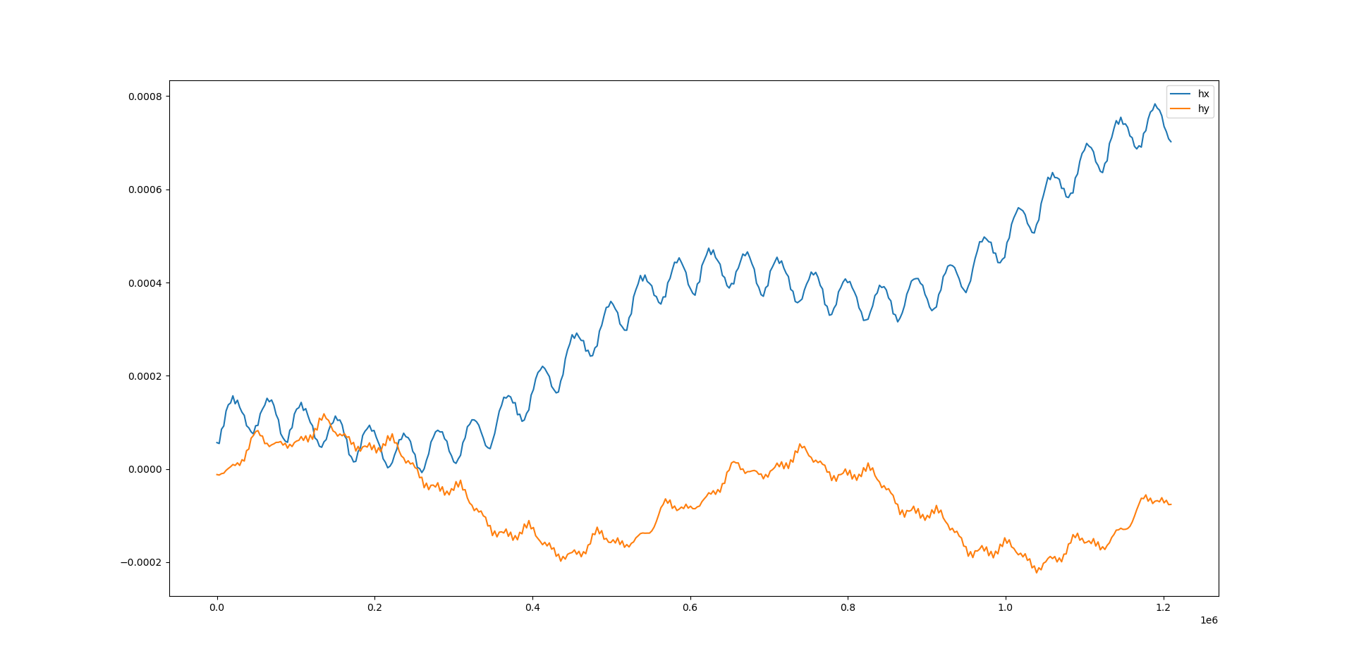
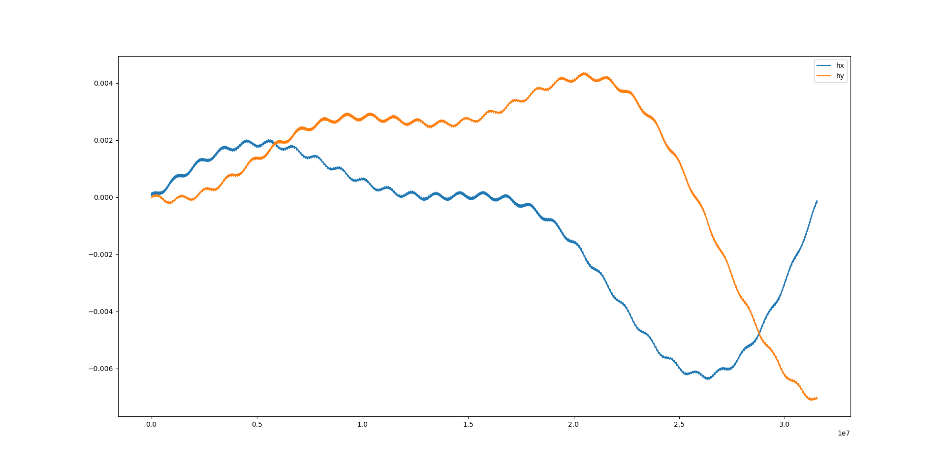
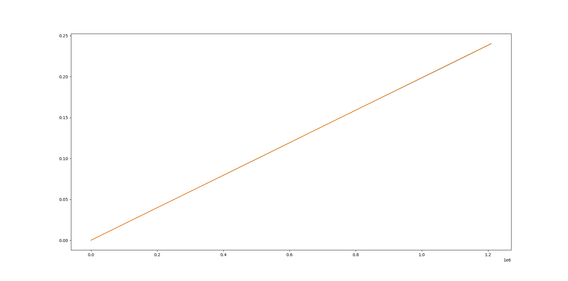
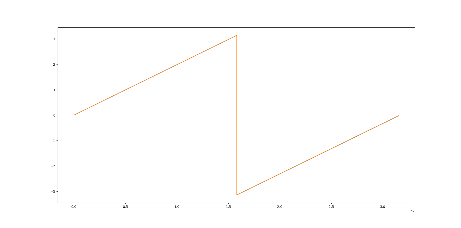
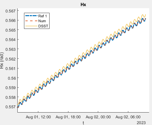
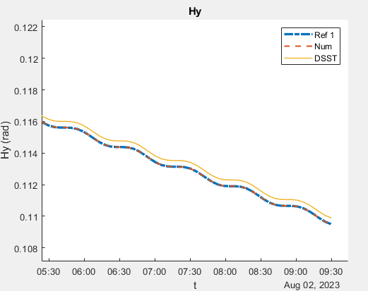
Could you please zoom in on hx/hy plots so that we can better see the differences between mean and osculating, and also plot the variation of right ascension at ascending node?
I also would like to mention that all these plots are generated considering only the geopotential expansion (4,4) as perturbing force. Indeed, by previous analyses I noticed that this is the term that causes this behaviour. Indeed, the DSSTPropagator was perfectly able to capture the dynamic evolution caused by the other perturbations. Moreover, this error becomes less and less visible with increasing altitude, again suggesting that the cause is the geopotential expansion.
Yes, that is my understanding. To be more precise, the only rigorous comparison are between osculating elements or between mean ones, but only when obtained straight by averaging the osculating ones according to the corresponding theory (so it can only be on the type of coordinates associated to it e.g. equinoctial for DSST). I think that anything else would in general introduce an “algebraic” error. That being said, it can be small, and maybe even negligible in many cases.
On another note, let’s keep in mind that the mean-to-osculating conversion (and the reciprocal by dependence) is only valid to a certain extent as there is always some approximation somewhere, in particular with complex perturbations. A good illustration is what Bryan said about Week Time Dependent terms in Orekit’s implementation of Third bodies. Also the second-order effects of J_2 are only available in the develop branch (have you tried it?). So you might just be seeing the limits of the DSST’s short-term geopotential, especially the tesseral harmonics given their simplified Earth rotation pointed out by Luc. It’s actually a shame (and perhaps not a coincidence) that we cannot simulate a 2x2 or 3x3 expansion.
I see, thanks for the explaination.
Also, thanks for pointing me towards some known issues about the DSST implementation. Maybe you’re right, and what I’m seeing is just another example of those issues. Honestly, I have no idea
BTW, no I haven’t tried the develop branch because I think that’s only available for the Java version, and unfortunately I’m not very good in Java, so I tend to stay away from it as much as I can
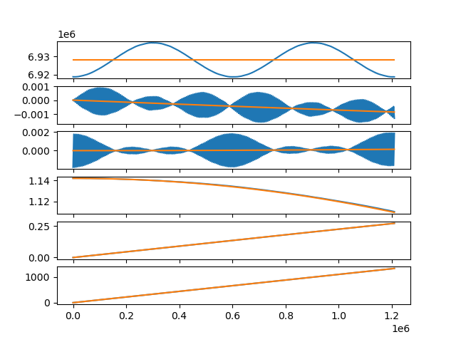
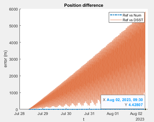
Is this still a problem in Orekit 11.3.2? I would say yes as I have been testing the DSST propagator to compare against a numerical one with similar perturbations, and adding the Harmonics (even just the J2) makes a big difference (at least when comparing the position):
I have checked the (Osculating) equinoctial elements to see where are the differences, and it appears to be mainly in Hx and Hy (this is after 5 days):
Some clarifications:
Ref 1 is a numerical orbit with the same perturbations, but with lower position tolerance (an order less than Num)
Only J2 is added of the Earth Harmonics
The atmosphere perturbation is the NRLMSISE00
The minStep of DSST is KeplerianPeriod/10, the maxStep = 100 * minStep, and positionTolerance is 10 times the position tolerance of Num
I have initial conditions in osculating elements (I define an orbit in keplerian elements, convert that to equinoctial, and use it to create the SpacecraftState for all propagators), and indicate that when I initialize the DSST propagator setInitialState. Also, I include PropagationType.OSCULATING in the creation of the DSSTPropagator to get the output in osculating elements and compare with the other propagators (I hope this does not create the type of errors in position that I am seeing…)
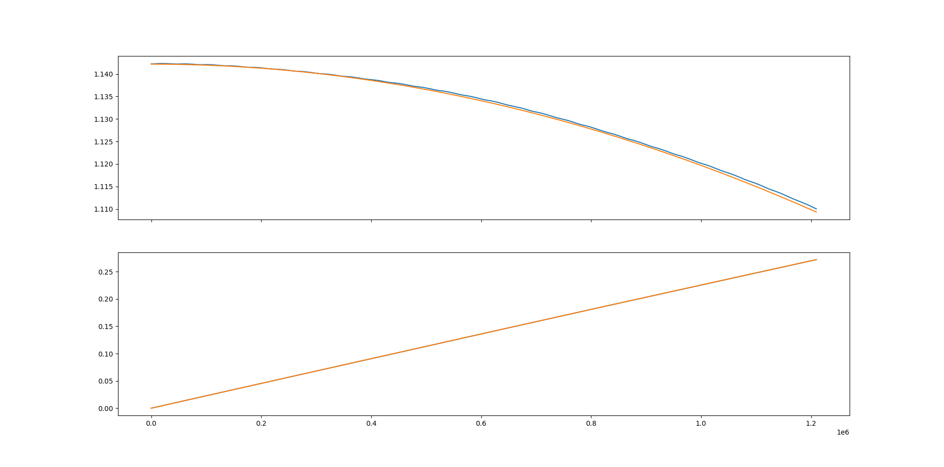
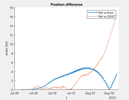
I have concluded that the problem, if there is one, has to be with the harmonics part of the propagation, without it I get:
which now could be attributed to the tolerances being greater, or just a product of the aproximation of the DSST theory (which I don’t completely understand at the moment).
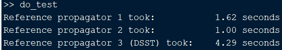
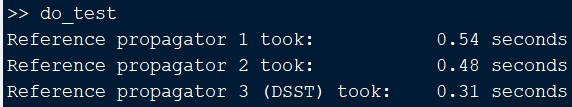
The purpose of these test are to find a compromise in the propagator that allows me to get faster approximations of the prediction for maneuver detection. And the most strange thing to me is that I am getting higher propagation times with the DSST:
I think the increase in computation comes only from the addition of the Atmosphere model (which is an empirical one and expensive to compute), but I don’t understand why it affects so much the DSST propagator. This are the computation times without atmosphere perturbation (the rest of the perturbations are Moon, Sun and SRP):
If it is the case that DSST has not changed in 11.3.2, and that 12.0 will inlcude the “fixes” for the difference with the numerical one, then I probably won’t be able to use it for my current project (I don’t know how to compile the develop branch for use in Matlab).
I recently opened issue 1104 related to the discrepancy in osculating elements.
Could you please share your initial orbit(s), force models etc. so we can reproduce your test.
Or a Junit test, that would be the best.
Yes the atmospheric drag computation is not very performant with DSST. Still, I’m surprised you get such an overhead with the DSST.
As you suspect, the J2 square thing will only be available in the next major release. This and other approximation/errors in the DSST model might explain the discrepancy.
As for performance, non conservative forces are treated by quadrature so should be much slower than the others. You should be able to tune the number of quadrature points if I’m not wrong.
Moreover, in my experience, if you require many intermediate points and you have many perturbations taken into account, propagation in osculating elements is computationally expensive. It can make you lose the time advantage gained by having large integration steps. If mean elements are enough for you, I would suggest propagating only them. Note also that I’m not sure what happens with DSST when you have events resetting the state or it’s derivatives e.g. impulsive maneuvers.
I would not recommend RESET_STATE with an osculating DSST until this behavior is fixed.
I have some leads on how to solve this but I’m not very happy with it yet.
I know there are a couple functions in there that are not specified anywhere, but one is for date conversion between Matlab and Orekit format, and the other is just a shortcut for calling the gravity field provider with the degree and order specified (either normalized or unnormalized). Aside from that is just a script for comparing the error in instantaneous position (and osculating elements) between DSST and a numerical propagator, all with the same perturbations (or I thought they were the same).
If something else is needed to reproduce the results just ask for it.
Thanks in advance.
Thank you @Serrof , actually this test was my first try at the DSST propagator so I really did not know what I would find. Actually, I don’t really need many intermediate points, but ploting many intermediate states between start and end of the propagation is always what I do when I want to get a feel at how the error grows. In reality I would only need the state (not in mean, but osculating) at the end of the propagation (and an estimation of the covariance, but that is another story), and wanted to see if this propagator would be a good alternative/compromise between precision and speed. For my application I need both the harmonics and a good atmosphere model (the orbits are too low to ignore those), so maybe this DSST propagator is not a good fit for my needs.
I was wondering if you fully solved the issue regarding inclination comparisons between DSST and numerical propagations.
It might be that the “problem” is indeed related to reference frames. In particular regarding gravity field zonal terms. In the DSST formulation the Zonal perturbations are added without specifying the Earth’s BF rotation axis, thus I would assume that the provided Zonal’s coefficients are implicitly associated to another axis, the one of the ECI frame, which by the way is fixed over time.
On the contrary, the same provided Zonal’s coefficients are correctly associated to the Earth’s (accurate) BF frame (e.g. ITRF) and thus takes into account variations of the axis over time.
A way to see this is to provide only J2 perturbation, and force the numerical propagator to associate it (e.g. the HolmesFeatherstoneAttractionModel) to the Inertial Frame.
On the one hand, the corresponding differences in position should not be much large. On the other hand, it would be interesting to investigate if it’s possible to include axis variations also in the DSST zonal perturbation term.
There’s issue 1104 on the forge whose partial fix is to introduce the rotating frame in zonal contribution.
There’s also draft merge request 507 that implements the feature you’re talking about.
I’d like to find some time to finish it…
In the meantime, I suggest you use the TOD inertial frame whose Z axis is closer to ITRF. This should remove most of the inclination drift.
thank you very much. Glad to hear you’re already working on it (I had actually missed your post with the issue 1104, sorry). Yes, I will also try with the TOD frame, I agree that it would improve the agreement in the inclination behaviors.