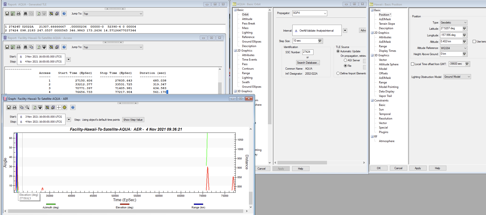
Okay here is a screen capture of the STK analysis. Sorry the elevation plot has Azimuth and Range (STK cant plot elevation alone). Note the elevation is above 5 deg (as part of the constraint). The first time at access is: 27150s from Epoch.
The contact Durations are: 685, 319, 634, 561 seconds.
Here is my modified code to the TLE_Propagation.ipynb:
I am not the best programmer, please don’t judge my elevation > 5 access time algorithm (or do, I love criticism). In summary:
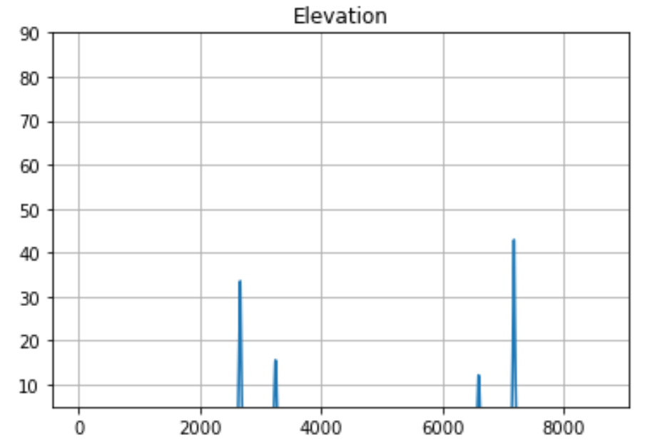
The first time at access is 26370s from Epoch
My contact durations are: 640, 510, 440, 660 seconds.
You can see that the elevation>5 peaks are near the same area, but have different maximums. It’s close but something is off.
`# Two Line Elements Propagation
## Authors
Petrus Hyvönen, SSC

## Learning Goals
* *Propagate an TLE*: Specify and read a TLE and propagate it with the orekit TLE propagator
* *Representation of ground station*: How to represent ground points
* *Elementary plotting in Python*: Simple ways to plot data

## Keywords
orekit, TLE, ground station

## Summary

This small tutorial is a first step to a real propagation of a satellite orbit
based on the common TLE format. The results are propagated in an inertial coordinate
system and then converted to a topocentric coordinate system, such as a ground station.

# Set up
%matplotlib inline
import numpy as np
## Initialize Orekit
Import orekit and set up the java virtual machine.
import orekit
vm = orekit.initVM()
Read the orekit-data file with basic paramters. This file is assumed to be in the current directory.
from orekit.pyhelpers import setup_orekit_curdir
setup_orekit_curdir()
Now we are set up to import and use objects from the orekit library.
from org.orekit.frames import FramesFactory, TopocentricFrame
from org.orekit.bodies import OneAxisEllipsoid, GeodeticPoint
from org.orekit.time import TimeScalesFactory, AbsoluteDate, DateComponents, TimeComponents
from org.orekit.utils import IERSConventions, Constants
from org.orekit.attitudes import AttitudeProvider, NadirPointing;
from org.orekit.propagation.analytical.tle import TLE, TLEPropagator
from math import radians, pi
import matplotlib.pyplot as plt
## Setting up the TLE
Specify the two line elements that describes the orbit of the satellite as strings. Here these are specified directly, in a larger example these would likely be fetched from a file or from an on-line service.
#AQUA27424 14th Oct 2021
# tle_line1 = "1 27424U 02022A   21287.75000000  .00000236  00000-0  52447-4 0 00007"
# tle_line2 = "2 27424 098.2183 227.4060 0000564 048.7337 097.6708 14.57117062034446"

# 3 Nov 2021
tle_line1 = "1 27424U 02022A   21307.66666667  .00000236  00000-0  52390-4 0 00004"
tle_line2 = "2 27424 098.2183 247.0537 0000565 346.9863 173.2636 14.57126477037344"

# GPS BIIF-2  (PRN 01)
# tle_line1 = "1 37753U 11036A   21307.14859678 -.00000068  00000-0  00000-0 0  9992"
# tle_line2 = "2 37753  56.4944  37.5291 0109002  50.1825 311.3781  2.00563888 75443"


The orekit TLE object parses the two line strings. [See TLE Doc](https://www.orekit.org/static/apidocs/org/orekit/propagation/analytical/tle/TLE.html) The Epoch is the timestamp where the two line elements are referenced to.
mytle = TLE(tle_line1,tle_line2)

print (mytle)
print ('Epoch :',mytle.getDate())

Epoch : 2021-11-03T16:00:00.000

## Preparing the Coordinate systems
Orekit supports several coordinate systems, for this example the International Terrestrial Reference Frame (ITRF) is used for the planet. A slightly elliptical body is created for the Earth shape, according to the WGS84 model.
ITRF = FramesFactory.getITRF(IERSConventions.IERS_2010, True)
earth = OneAxisEllipsoid(Constants.WGS84_EARTH_EQUATORIAL_RADIUS,
                         Constants.WGS84_EARTH_FLATTENING,
                         ITRF)
## Define the station
The location of the station is defined, and a [TopocentricFrame](https://www.orekit.org/site-orekit-10.1/apidocs/org/orekit/frames/TopocentricFrame.html) specific for this location is created.

This frame is based on a position near the surface of a body shape. The origin of the frame is at the defining geodetic point location, and the right-handed canonical trihedra is:

- X axis in the local horizontal plane (normal to zenith direction) and following the local parallel towards East
- Y axis in the horizontal plane (normal to zenith direction) and following the local meridian towards North
- Z axis towards Zenith direction
longitude = radians(27.5207)
latitude  = radians(-157.996)
altitude  = 0.402*1000 #m
station = GeodeticPoint(latitude, longitude, altitude)
station_frame = TopocentricFrame(earth, station, "Esrange")
For the propagation a Earth centered inertial coordinate system is used, the EME2000. This frame is commonly also called J2000. This is a commonly used frame centered at the Earth, and fixed towards reference stars (not rotating with the Earth).
inertialFrame = FramesFactory.getEME2000()

# satelliteFrame = FramesFactory.getGCRF()
# attitudeProvider = NadirPointing(satelliteFrame, earth)
# propagator = TLEPropagator.selectExtrapolator(mytle,attitudeProvider,3117,FramesFactory.getTEME())

propagator = TLEPropagator.selectExtrapolator(mytle)
Set the start and end date that is then used for the propagation.
#14th october 2021
# extrapDate = AbsoluteDate(2021, 10, 14, 18, 0, 0.0, TimeScalesFactory.getUTC())
# finalDate = extrapDate.shiftedBy(60.0*60*24) #seconds

# 3 Nov 2021 16:00:00.000 UTCG
extrapDate = AbsoluteDate(2021, 11, 3, 16, 0, 0.0, TimeScalesFactory.getUTC())

#  Epoch : 2021-11-03T03:33:58.762
# extrapDate = AbsoluteDate(2021, 11, 3, 3, 33, 58.762, TimeScalesFactory.getUTC())

finalDate = extrapDate.shiftedBy(60.0*60*24) #seconds

print(extrapDate)
print(finalDate)
el=[]
pos=[]
contactTime = []
index=0

endAccessTime = []
endAccessTimeIndex = []
epochTime = []
epochTime_tmp = 0.0
accessTime = []

stepsize_s = 10.0

while (extrapDate.compareTo(finalDate) <= 0.0):
    pv = propagator.getPVCoordinates(extrapDate, inertialFrame)
    pos_tmp = pv.getPosition()
    pos.append((pos_tmp.getX(),pos_tmp.getY(),pos_tmp.getZ()))

    el_tmp = station_frame.getElevation(pv.getPosition(),
                    inertialFrame,
                    extrapDate)*180.0/pi
    el.append(el_tmp)
    extrapDate = extrapDate.shiftedBy(stepsize_s)

    epochTime_tmp += stepsize_s
    epochTime.append(epochTime_tmp)


    if el_tmp > 5:

        accessTime.append(epochTime_tmp)

        if accessTime[index] - accessTime[index-1] > stepsize_s:
            # endAccessTime.append(epochTime_tmp)
            endAccessTimeIndex.append(index-1)


        index += 1
print(len(endAccessTimeIndex))

for ii in range(len(endAccessTimeIndex)+2):
    if len(endAccessTimeIndex) != 0:
        if ii == 0:
            contactTime.append(accessTime[endAccessTimeIndex[ii]]-accessTime[0])
        elif ii == len(endAccessTimeIndex)+1:
            contactTime.append(accessTime[-1]-accessTime[endAccessTimeIndex[ii-2]+1])

        elif ii < 3:
            # print(ii)
            # print(accessTime[endAccessTimeIndex[ii]]-accessTime[endAccessTimeIndex[ii-1]+1])
            contactTime.append(accessTime[endAccessTimeIndex[ii]]-accessTime[endAccessTimeIndex[ii-1]+1])
    else:
        contactTime=accessTime[-1]-accessTime[0]


## Plot Results
Plot some of the results from the propagation. Note that in the plots below the x-axis are samples and not proper time.
for ii in range(len(contactTime)):
    print("The Contact Time for Access #{} is {} s.".format(ii,contactTime[ii]))
print("The total contact time is {} s.".format(sum(contactTime)))
print(accessTime[0])


The Contact Time for Access #0 is 640.0 s.
The Contact Time for Access #1 is 510.0 s.
The Contact Time for Access #2 is 440.0 s.
The Contact Time for Access #3 is 660.0 s.
The total contact time is 2250.0.
[26370.0]

# print(max(el))

plt.plot(el)
plt.ylim(5,90)
plt.title('Elevation')
plt.grid(True)
plt.plot(pos);
plt.title('Inertial position');


`